The immediate aim of validphys2 is to serve as a both very agile and highly reliable analysis framework for NNPDF, but the goal extends beyond. When the time codes, this framework should become the common gateway that all the NNPDF code uses, providing features ranging from path handling to automated report generation to automatic detection of problems with the fits.
The project is defined in two codes with well defined and separated scopes:
pandoc program to generante a HTML report. Apart from the compiler functionality, reportengine also provides general application utilities such as crash handlers and a help system.
reportengine application or standalone. It is based on the libnnpdf Python wrappers, and extends them with extra functionality (related to error checking, loading and downloading among others). The NNPDF objects are then used in functions producing plots, tables and other outputs (such as reweighted PDF sets)
Right now the following features are implemented:
These features are documented in more detail in Usage.
A scientific program usually requires a large set of complex input parameters and can take a very long time to produce results. Results tend to be frequently unexpected even if everything is working correctly. It is essential to check that the inputs are correct and make sense. Also, the inputs of a given function should be checked as early as possible, which is not necessarily at the point of the program where the function is to be called. For example, something like this:
def check_parameter_is_correct(parameter):
    ...

def plot(complex_calculation, parameter):
    check_parameter_is_correct(parameter)
    #make plot
    ...
has the disadvantage that in order to get to the check, we presumably need to compute “complex_calculation” first, and that could be a waste of time if it turns out that “parameter” is not correct for some reason and we can’t do the plot anyway. Instead we should arrange to call “check_parameter_is_correct(parameter)” as early as possible (outside the plotting function) and show the user an informative error message.
Of course it is impossible to guarantee that this is always going to happen. For example it is possible that we check that a folder exists and we have permissions to write to it, but by the time we actually need to write, the folder has been deleted. However in such cases the state of the program can be considered broken and it’s OK to make it fail completely.
There is an API for early checks in reportengine. We would write something like:
@make_argcheck
def check_parameter_is_correct(parameter):
    ...

@check_parameter_is_correct
def plot(complex_calculation, parameter):
    #make plot
    ...
The checking function will now be called as soon as the program realizes that the plot function will be required eventually (at “compile time”). The user would be shown immediately an error message explaining why the parameter is wrong.
The fancy term for this style of coding is Contract Programming.
It is extremely convenient to be able to specify the what the program should only without any regard of knowledge of how that is achieved by the underlying implementation. The current nnfit input files are a good example of this. The primary input of validphys are YAML run cards. A very simple one looks like this:
pdfs:
    - NNPDF30_nlo_as_0118
    - NNPDF30_nnlo_as_0118
    - CT14nlo

first:
    Q: 1
    flavours: [up, down, gluon]

second:
    Q: 100
    xgrid: linear

actions_:
    - first:
        - plot_pdfreplicas:
            normalize_to: NNPDF30_nlo_as_0118

        - plot_pdfs
    - second:
- plot_pdfreplicasA declarative input specifies what you want. It is up to the underlying code to try to provide it (or fail with an informative message).
It is easy for a human to verify that the input is indeed what it was intended. Even without any explanation it should be easy enough to guess what the runcard above does.
The input is very loosely coupled with the underlying implementation, and therefore it is likely to remain valid even after big changes in the code are made. For example, in the runcard above, we didn’t have to concern ourselves with how LHAPDF grids are loaded, and how the values of the PDFs are reused to produce the different plots. Therefore the underlying mechanism could change easily without breaking the runcard.
Therefore:
While the goal of reportengine is to allow simple and easily repeatable bach actions, sometimes it is far simpler to get the work done with a raw (Python) script, or it is needed to explore the outcomes using something like an IPython notebook. It would be good to be able to use all the tools that already exist in validphys for that, without needing to reinvent the wheel or to alter functions so that for example they don’t to some preconfigured path. Therefore:
This is implemented by making sure that as much as possible all the validphys functions are pure. That is, the output is a deterministic function of the inputs, and the function has no side effects (e.g. no global state of the program is altered, nothing is written to disk). There are some exceptions to this though. For example the function that produces a reweighted PDF set needs to write the result to disk. The paths and side effects for other more common results like figures are managed by reportengine. For example, the @figure decorator applied to a function that returns a Python (matplotlib) figure will make sure that the figure is saved in the output path, with a nice filename, while having no effect at all outside the reportengine loop. The same goes for the check functions described above.
Very frequently there is the need to compare. It is easy enough to write simple scripts that loop over the required configurations, but that cannot scale well when requirements change rapidly (and is also easy to make trivial mistakes). Therefore reportengine allows configurations to easily loop over different sets of inputs. For example the following runcard:
pdfs:
    - id:  160502-r82cacd2-jr-001
      label: Baseline

    - id: 160502-r82cacd2-jr-008
      label: HERA+LHCb

    - id: 160603-r654e559-jr-003
      label: baseline+LHCb and Tev legacy

fit: 160603-r654e559-jr-003
theoryids:
    - 52
    - 53
use_cuts : False

experiments:
  - experiment: LHCb
    datasets:
      - { dataset: LHCBWZMU7TEV, cfac: [NRM] }
      - { dataset: LHCBWZMU8TEV, cfac: [NRM] }

  - experiment: ATLAS
    datasets:
      - { dataset: ATLASWZRAP36PB}

actions_:
 - theoryids:
    pdfs:
        experiments:
            experiment:
              - plot_fancy
Will produce a separate plot for each combination of the two theories (52 and 53), the three pdfs at the top, and each dataset in the two experiments (so 18 plots in total). This syntax is discussed in more detail in the Usage section.
The requirements above (in particular the combination of early checking and arbitrary looping) lead to the condition that the value of the resources depends on the other resources involved. For example, a dataset requires a theoryid in order to locate the FKTables and cfactors, and we want to check that these paths exist early on.
Therefore the processing always starts from the user requirement (i.e. the requested actions) and processes each requirement for that action within the correct context, trying to avoid duplicating work. Conversely we ignore everything that is not required to process the actions.
A lot of work has gone into producing a usable installer that works on both Linux and Mac. Currently the installation for both platforms boils down to executing a script.
Producing installers is a difficult (and boring) problem since a lot of dependencies needs to be set up to work properly together. In practice, it is hard to produce a set of instructions that work reliably on all platforms and with all compilers. This is further complicated by the fact that the Python deployment tools are substandard in several ways (such as avoiding unwanted interaction between libraries for Python 2 and Python 3). Furthermore, on Mac gcc and clang interact poorly when it comes to including the C++ standard library, and a lot of care has to be taken to include the correct one.
The solution to all that is to provide precompiled versions of all the dependencies, that are generated automatically when new commits are pushed to the CERN Gitlab server (for Linux) and the Travis CI server (for Mac).
The compiled binaries are subsequently packaged (using conda) and uploaded to a remote server where they are accessible. These packages are known to compile on clean default environments (namely those of the CI servers used to produce the packages), and the Python packages are known to be importable. Everything that an user has to do is to configure conda correctly and ask it to install the validphys2 package with all its dependencies. This results in an environment that contains not only an usable version of validphys, but also of the nnpdf code and all its dependencies (including for example LHAPDF and APFEL). Therefore an user who doesn’t need to modify the code should not need to compile anything to work with the NNPDF related programs. This should be useful in clusters where we don’t completely control the environment and frequently need to deal with outdated compilers.
A helper script exists to aid the configuration. All you need to do is:
#Obtain the helper script
git clone ssh://git@gitlab.cern.ch:7999/NNPDF/binary-bootstrap.git
#Execute the script
./binary-bootstrap/bootstrap.sh
The script will ask for the password of the NNPDF private repositories. You can find it here:
https://www.wiki.ed.ac.uk/pages/viewpage.action?spaceKey=nnpdfwiki&title=Git+repository+instructions
The conda installer will ask to add the conda bin path to the default $PATH environment variable (by editing your .bashrc file). Confirm this unless you know that you have a specific reason not to.
Not that the script may ask you to perform some actions manually (e.g. it will not overwrite your existing conda configuration). Please be pay attention to the output text of the script.
Once everything is configured, you can install validphys and nnpdf by simply running:
conda install validphys nnpdfThere is only one thing left to do. We don’t package the nnpdfcpp data in the conda packages (that would make them too big) and furthermore the binaries expect to be operated from specific relative paths with respect to the data. To work around these limitations we can symlink the nnpdfcpp binaries to the correct path, which is a bin/ folder inside the root of the nnpdfcpp git repository.
```cd nnpdfcpp mkdir -p bin && cd bin #inside nnpdfcpp/bin ln -s which nnfit . ln -s which postfit . ln -s which fitmanager . ln -s which chi2check . ``` This requirement will disappear in the future. See also Dealing with paths below.
Note this is not required for validphys to work.
After several iterations on the install system most issues have been resolved. There could be problems derived from interactions with hacks targeted at solving manually. In particular, see that you don’t have any PYHTONPATH environment variable (for example pointing at some version of LHAPDF) since that will overwrite the default conda configuration. This is easily solved by removing said hacks from .bashrc or similar files.
If you include conda in your default PATH, the default Python version will be the conda Python 3. This could cause problems if you use code that expects /usr/bin/env python to point to Python 2. In such cases you will need to conditionally enable or disable conda. You can saved a helper executable script (called for example use-conda) to some location in your PATH containing:
#!/bin/bash
unset PYTHONPATH
export PATH= /your/conda/folder/bin:$PATH
Remember to chmod +x use-conda. Now typing:
source use-condawill set your PATH environment variable to point to the conda binaries.
In any case this tends to not be a problem for newer software as Python 3 gains support.
You can conda install a package and then conda remove --force it to obtain an environment with all the dependencies but without the package. Then for Python projects you can use pip install -e . in the root folder where the setup.py folder is located to have the environment automatically reflect the changes you make to the files. For example, if you wanted to develop the validphys code you would do:
#Quickest way to get all the dependencies in place
conda install validphys
conda remove validphys --force

git clone ssh://git@gitlab.cern.ch:7999/NNPDF/validphys2.git
cd validphys2
pip install -e .
For C++ projects use the usual build systems, setting the prefix to the conda folder.
A help command is generated automatically by reportengine. The command
validphys --helpwill show you the modules that contain the actions (as well as the usual description of the command line flags). For example,
validphys --help validphys.plotswill list all the actions defined in the plots module together with a brief description of each of them. Asking for the help of one of the actions, like for example:
validphys --help plot_fancywill list all the inputs that are required for this action. For example the command below results currently in the following output:
plot_fancy

Defined in: validphys.plots

Generates: figuregen

plot_fancy(one_or_more_results, dataset, normalize_to:(<class 'int'>,
  <class 'str'>, <class 'NoneType'>)=None)

Read the PLOTTING configuration for the dataset and generate the
corrspondig data theory plot.

The input results are assumed to be such that the first one is the
data, and the subsequent ones are the predictions for the PDFfs. See
``one_or_more_results``. The labelling of the predictions can be
influenced by setting ``label`` attribute of theories and pdfs.

normalize_to: should be either 'data', a pdf id or an index of the
result (0 for the data, and i for the ith pdf). None means plotting
absolute values.

See docs/plotting_format.md for details on the format of the PLOTTING
files.

The following resources are read from the configuration:

    dataset(dict): Dataset specification from the theory and
  CommonData. Use the cuts from the fit, if provided.

    theoryid: A number corresponding to the database theory ID where
  the corresponding theory folder is installed in te data directory.
  Either just an id (str or int), or a mapping with 'id' and 'label'.
  [Used by dataset]

    use_cuts(bool): Whether to use the filtered points in the fit, or
  the whole data in the dataset.
  [Used by dataset]

    fit: A fit in the results folder, containing at least a valid
  filter result. Either just an id (str), or a mapping with 'id' and
  'label'.
  [Used by dataset]

    pdfs(list): A list of pdf objects.
  [Used by one_or_more_results]

    pdf: A PDF set installed in LHAPDF. Either just an id (str), or a
  mapping with 'id' and 'label'.
  [Used by one_or_more_results]

    use_t0(bool): Whether to use the t0 PDF set to generate
  covariance matrices.
  [Used by one_or_more_results]

    t0pdfset: PDF set used to generate the t0 covmat.
  [Used by one_or_more_results]

The following additionl arguments can be used to control the
behaviour. They are set by default to sensible values:

  normalize_to(int or str or NoneType) = None
We can see which keys have a special meaning in the configuration file with:
validphys --help configAll other keys are interpreted literally (although they could be further processed by specific actions).
At the moment nnpdfcpp and the resources it contains (such as fits and datasets) don’t adhere to any common PREFIX specification, and instead rely on complicated relative paths relations to localize the resources. While this probably needs to be changed eventually, replaced by some more robust and standard solution, there is no way for validphys to work other than to behave the same way at the moment.
By default, it is assumed that validphys is executed inside a folder at the same level as “nnpdfcpp”. Otherwise, the --datapath should be set to point to nnpdfcpp/data and --resultspath should point to a folder containing the fits.
This is extremely annoying and will be changed in the near future.
Input cards are YAML files that describe the input resources, together with the actions we want to perform on them.
Let’s begin with a simple example:
pdf: NNPDF30_nlo_as_0118

theoryid: 52

use_cuts: false

dataset:
    dataset: ATLASWZRAP36PB
    sys: 2
    cfac: [EWK]

actions_:
  -   - plot_fancy
      - plot_chi2dist
We are specifying one PDF (by the LHAPDF id), one dataset and one theory. Npte that the dataset specification is identical to that of the nnfit configuration files. We are saying that we do not want to use the cuts of the data (so we don’t have to specify a fit containing the cut data).
The special actions_ key is used to declare the actions we want to have executed. We want a data/theory comparison (plot_fancy) and to plot the distribution of the chi² for each replica (plot_chi2dist). If we save the above runcard to a file called runcard.yaml we can produce the plots with:
validphys runcard.yamlResources can be declared at top level, like in the example above, inside a mapping (with an arbitrary key), or inside an element of a list of mappings.
For example, we can modify the example as follows:
pdf: NNPDF30_nlo_as_0118

theoryid: 52

fit: 161222-jr-004

with_cuts:
  use_cuts: True

without_cuts:
  use_cuts: False

dataset:
    dataset: ATLASWZRAP36PB
    sys: 2
    cfac: [EWK]

actions_:
  - with_cuts:
      - plot_fancy

  - without_cuts:
      - plot_chi2dist
Here with_cuts and without_cuts are arbitrary strings that specify namespaces. Now we are asking for one action (plot_fancy) to be executed taking into account the cuts (note that we have also specified the fit where we read them from) and another (plot_chi2dist) to be executed without the cuts. Similar to a programming language like C, the inner namespaces has priority with respect to the outer. For example if we add a PDF specification to the “with_cuts” namespace like this:
pdf: NNPDF30_nlo_as_0118

theoryid: 52

fit: 161222-jr-004

with_cuts:
  use_cuts: True
  pdf: CT14nlo

without_cuts:
  use_cuts: False

dataset:
    dataset: ATLASWZRAP36PB
    sys: 2
    cfac: [EWK]

actions_:
  - with_cuts:
      - plot_fancy

  - without_cuts:
      - plot_chi2dist
The plot_fancy action will ignore the outer pdf (NNPDF30_nlo_as_0118) and use the one defined in the innermost namespace (CT14nlo). Because we have not specified plot_chi2dist to be executed within the with_cuts namespace, it will continue to use NNPDF.
We can also have lists of mapping acting as namespaces. The action will then be repeated inside each of the namespaces generating one result for each. For example:
pdf: NNPDF30_nlo_as_0118

theoryid: 52

fit: 161222-jr-004

specifications:
- use_cuts: True
  pdf: CT14nlo

- use_cuts: False

dataset:
    dataset: ATLASWZRAP36PB
    sys: 2
    cfac: [EWK]

actions_:
  - specifications:
      - plot_fancy
Now a different plot_fancy action will be executed for each of the two mappings of the list “specifications”: One will use the CT PDF and use the cuts, and the other will plot all points in the dataset.
Some keys are appropriately interpreted either as lists of objects or list or namespaces depending on the context. They are documented in validphys --help config. For example, the pdfs key is entered as a list of LHAPDF ids:
pdfs:
  - NNPDF30_nlo_as_0118
  - CT14nlo
Because the plot_fancy action takes a list of pdfs as input, something like this:
pdfs:
  - NNPDF30_nlo_as_0118
  - CT14nlo

theoryid: 52

use_cuts: False

dataset:
    dataset: ATLASWZRAP36PB
    sys: 2
    cfac: [EWK]

actions_:
  - - plot_fancy
will produce plots where the two pdfs appear together. However we can also produce individual plots for each pdf, by simply specifying that we want to loop over the pdfs:
pdfs:
  - NNPDF30_nlo_as_0118
  - CT14nlo

theoryid: 52

use_cuts: False

dataset:
    dataset: ATLASWZRAP36PB
    sys: 2
    cfac: [EWK]

actions_:
  - pdfs:
      - plot_fancy
In this case the value of the pdfs key is seen as equivalent to:
pdfs:
  - {pdf: NNPDF30_nlo_as_0118}
  - {pdf: CT14nlo}
However the special treatment allows us to simplify both the input file and the programmatic interface of the functions (see Automatic Lists).
Namespace specifications like those described above can be arbitrarily nested. Values will be searched from inner to outer namespace. When the namespace specifications represent lists of mappings, all possible combinations will be produced.
Consider the example:
pdfs:
    - 160502-r82cacd2-jr-001

    - 160502-r82cacd2-jr-008

    - 160603-r654e559-jr-003

fit: 160603-r654e559-jr-003
theoryids:
    - 52
    - 53

with_cuts:
    use_cuts : False

experiments:
  - experiment: LHCb
    datasets:
      - { dataset: LHCBWZMU7TEV, cfac: [NRM] }
      - { dataset: LHCBWZMU8TEV, cfac: [NRM] }

  - experiment: ATLAS
    datasets:
      - { dataset: ATLASWZRAP36PB}

actions_:
    - with_cuts:
        theoryids:
          pdfs:
            experiments:
                experiment:
                  - plot_fancy
This will first enter the “with_cuts” namespace (thus setting use_cuts=False for the action), and then loop over all the theories, pdfs, experiments and datasets inside each experiment (note that when used as a namespace specification, experiment refers to the list of datasets it contains).
The order over which the looping is done is significative: For one the outer specifications must set all the variables required for the inner to be fully resolved (so with_cuts must go before experiment).
For other, the caching mechanism works by grouping together the namespace specifications from the beginning. For example, suppose we where to add another action to the example above:
    - with_cuts:
        theoryids:
          pdfs:
            experiments:
                experiment:
                  - plot_chi2dist
both of these require to compute the same convolutions. Validphys will realize this as long as both actions are iterated in the same way. However permuting “pdfs” and “theotyids” would result in the convolutions computed twice, since the code cannot prove that they would be identical.
Always loop from more general to more specific.
Always loop in the same way.
Action arguments are syntactic sugar for specifying arguments visible to a single actions. They are subject to being verified by the action defined checks. For example, in the PDF plotting example above:
pdfs:
    - NNPDF30_nlo_as_0118
    - NNPDF30_nnlo_as_0118
    - CT14nlo

first:
    Q: 1
    flavours: [up, down, gluon]

second:
    Q: 100
    xgrid: linear

actions_:
    - first:
        - plot_pdfreplicas:
            normalize_to: NNPDF30_nlo_as_0118

        - plot_pdfs
    - second:
        - plot_pdfreplicas
The normalize_to key only affects the plot_pdfreplicas action. Note that defining it inside the first mapping would have had the same effect in this case.
from_ special keyThe from_ specifies that the value of a resource is to be taken from a container. This is useful for working with fits (but not limited to that). For example:
fit: 161208-jr-003

use_cuts: False

description:
    from_: fit

theory:
    from_: fit

theoryid:
    from_: theory


Q: 10

template: report.md

normalize:
    normalize_to: 1

datanorm:
    normalize_to: data

pdfs:
    - from_: fit
    - NNPDF30_nlo_as_0118
experiments:
    from_: fit

actions_:
   -   - report:
            out_filename: index.md
Here the from_ key is used multiple times:
To obtain the description string from the report input card.
To obtain the theory mapping from the fit input card.
To obtain the theoryid key from the theory mapping.
To obtain a single PDF produced in the fit (as an element of the list/namespaces of pdfs). Note that the keyword is also allowed inside nested elements.
To obtain a set of all the experiments of the fit.
The from_ key respects lazy processing, and therefore something like this will do what you expect:
fits:
    - fit: 161208-jr-003
    - fit: 161222-jr-004


use_cuts: False

theory:
    from_: fit

theoryid:
    from_: theory


Q: 10

description:
    from_: fit
template: report.md

normalize:
    normalize_to: 1

datanorm:
    normalize_to: data

pdfs:
    - from_: fit
    - NNPDF30_nlo_as_0118
experiments:
    from_: fit

actions_:
    - fits:
        - report
This will work exactly as the example above, except that a new action (with its corresponding different set of resources) will be generated for each of the two fits.
Several resources (PDFs, theories, fits) support a short form where one specifies the ID required to recover the resource (e.g. LHAPDF ID, theory ID and fit folder respectively) and also form where a plotting layer is specified together with the ID. For example:
pdfs:
    - id:  160502-r82cacd2-jr-001
      label: Baseline

    - id: 160502-r82cacd2-jr-008
      label: HERA+LHCb

    - id: 160603-r654e559-jr-003
      label: baseline+LHCb and Tev legacy
In all plots the label will be used everywhere the PDF name needs to be displayed (like in legends and axes).
Reports are implemented as an action of reportengine (admittedly a little hacky at the moment). The report action takes a template argument, corresponding to the filename of a template in the Pandoc Markdown format, with the actions defined with a special syntax discussed below. The actions will be resolve as if they where directly specified in the configuration file file, and when all of them are completed, their value will be substituted in the template (the jinja2 library is used for the intermediate rendering).
reportengine will interpret strings between {@ and @} inside the templates. There are currently target and with/endwith tags:
Specify an action to be executed. The possible syntax is:
{@[spec] action_name[(arg1=value, arg2=value)]@}where [] stands for optional syntax. A few conforming examples are:
{@ plot_fancy @}{@theory::pdfs plot_fancy@}{@plot_fancy(normalize_to=data)@}:: operator (resembling the C++ scope resolution operator). Actions will be repeated if the specification results in multiple namespaces (e.g. one plot per pdf in the second example above). The optional argument specification works as described in Action arguments.
Repeat the content between the tags for each namespace in the specifications. Targets inside the block are repeated and searched within each namespace. The syntax of the with tag is:
{@with spec@}and it must be closed by an endwith tag
{@endwith@}::.
A template that could correspond to the example above is:
NNPDF Report
============

{@ description  @}


PDF plots
---------

{@ plot_pdfs @}

**Normalized**

{@normalize plot_pdfs  @}


Train-valid split
------------------

{@ plot_training_validation @}

$\chi^2$
-------
{@ with pdfs  @}

### {@ pdf @}

{@ experiments_chi2_table @}

{@ endwith@}

Experiment plots
---------------
{@ with pdfs @}
###Experiment results for {@pdf@}
{@with datanorm::experiments@}

#### {@experiment@}
{@experiment plot_fancy @}
{@ endwith @}
{@ endwith @}
First we are writing a verbatim Markdown title. Next we are asking for a variable named “description” to be computed and later substituted right below (it is obtained from the fit config file, as seen in the template). Then we are computing absolute and normalized PDF plots (normalize is an arbitrary string that is defined in the config file to normalize to the first PDF). We then plot the training and validation χ2 of each replica in the fit. Next we compute the χ2 for each experiment, and produce a separate table and heading for each PDF in pdfs (note that LaTeX math syntax is allowed). Finally we produce, for each pdf and for each experiment, a set of data-theory comparison plots (which in turn are repeated for each dataset in the experiment).
There are too many tools that are still evolving too rapidly to completely document in here. Refer to the automatically generated command line help (Seeing what actions are available) for more up to date documentation. Here we only cover the complex tools that require more specific documentation.
The name of the data-theory comparison tool is plot_fancy. You can see what parameters in the runcard influence it by typing:
validphys --help plot_fancyThe basic inputs are a dataset and one or more PDFs. The way a dataset is to be plotted is controlled by one or more PLOTTING files in the commondata format. These are simple YAML files and ideally each dataset should have them. It is possible to specify how to transform the kinematics stored in the commondata, what to use as x axis or how to group the plots. The format is described in detail in Plotting format specification. The plotting specifications are supported by small amounts of Python (defining the varios transformations), which are declared in the validphys.plotoptions package.
It is possible to run validphys using all the available cores in the system. This is done simply using the --parallel flag. This will result in a performance gain for many run configurations. The parallel mode will be eventually enabled by default, and you can disable it explicitly with the --no-parrallel flag.
By default theories, fits and PDFs that are required will be downloaded automatically. PDFs are searched both in LHAPDF and in our custom fits. This can be controlled with the --net (no effect by default) and --no-net (disable all remote downloading) options. Because defaults could change in the future, it is useful that scripts calling validphys specify this behaviour explicitly.
Using the --upload flag, the contents of the output folder will be uploaded to the pcteserver, after validphys is done. An authorized ssh key and the rsync program are required in order to use this feature. A URL will be displayed from which the contents are publicly accessible.
All the uploaded results are automatically indexed in the server. Some metadata (e.g. author, and title) will be obtained from an index.html file in the uploaded output folder. To configure the report action to produce such metadata, set the out_filename option to index.html and use the pandoc-maarkdown syntax to set the metadata at the top of the file. In the runcard you would write something like:
template: mytemplate.md
actions_:
  -   - report:
          out_filename: index.html
and you would begin mytemplate.md like:
%My title: Testing fit {@ fit @}
% Zahari Kassabov
Note that you can use the report syntax to get the parameters from the runcard.
The output figure formats can be controlled with the --formats option. The available formas depend on the underlying implementation. On Linux with Anaconda, they are:
png: Portable Network Graphics
pdf: Portable Document Format
ps: Postscript
jpg: Joint Photographic Experts Group
rgba: Raw RGBA bitmap
eps: Encapsulated Postscript
tiff: Tagged Image File Format
raw: Raw RGBA bitmap
svg: Scalable Vector Graphics
pgf: PGF code for LaTeX
tif: Tagged Image File Format
svgz: Scalable Vector Graphics
jpeg: Joint Photographic Experts Group
The --formats option accepts more than one format. However if an HTML report is desired, one should make sure that the first format is browser friendly and can be displayed nicely without plugins (from the formats above, the browser friendly ones would be png, jpg, and svg).
Many of the options of matplotlib (the library we for plotting) can be controlled with a plotting style file. To customize (or “improve”) the looks of the plots, you can edit the validphys style src/validphys/small.mplstlye or pass your own style file with the --style option.
By default we try to only display useful information that the user should definitively read. In case something is not working correctly, debug messages can be enabled with the -d (or --debug) flag. More messages can be suppressed using the -q (or --quiet) flags. Additionally the messages from libnnpdf can be controlled with the --cout/--no-cout flags (by default the output is displayed only when the debug flag is enabled).
Validphys2 aims to be a simple and easy to extend framework, which is mostly elemental Python, with a couple of magic decorators that make reportengine work as expected. It should be relatively straightforward to understand and extend. How to do so is described in the Defining custom pipelines section.
Unfortunately this means that the complexity of getting things to just work is translated into reportengine, which instead uses many advanced python features, and results in a codebase that is not particularly simple.
A central concept to how reportengine works is namespaces and namespace specifications. A namespace is a stack of python dictionaries indexed by a tuple called namespace specification (nsspec). Nsspecs are generated from user input given in terms of fuzzyspecs. This is mostly an advanced internal implementation detail, but it is important in order to understand how several features work. Also the abstraction leaks into user facing features such as The collect function.
An nsspec is a tuple of an arbitrary number of elements. Each element in the tuple corresponds to one extra stack layer in depth (“stack frame”). The elements of the tuple can be either:
Names of mappings.
Names of objects that have an as_namespace method.
Tuples of the form (name of list of mappings, index).
The scope rules are similar to those of C: The lookup of a value is done first looking at the inner frame and then at the outer ones, until a match is found.
Consider the example:
first:
   pdf: NNPDF30_nlo_as_0118
   normalize_to: None
   use_cuts: False

second:
   pdf: CT14nlo
   normalize_to: CT14nlo

cutspecs:
 - {use_cuts: False}
 - {use_cuts: True}
Given the input above, we could form the following nsspec.
('second', ('cutspecs', 0))This would correspond to a namespace where we have the following symbols available:
use_cuts (set to False) from cutspecs.
pdf and normalize_to (set to CT) from second.
first, second and cutspecs from the root namespace.
We could also form the specification:
(('cutspecs', 1), 'first')Because the innermost specification is last, the value of use_cuts is False.
The function reportengine.namespaces.resolve(ns, nsspec) returns a mapping (in particular it is a modified version of collections.ChainMap) that implements exactly this behaviour. It is used extensively thorough reportengine.
The namespace specifications as described above is not what the user typically enters. Instead the typical user input is what in the code is labeled fuzzyspec. A fuzzyspec is like a nsspec except that the lists of mappings are entered by name and not by a tuple (name, index). A fuzzyspec resolves to one or more nsspecs. For example, given the fuzzyspec:
('second', 'cutspecs')and the input above, it gets expanded into two nsspecs:
('second', ('cutspecs', 0))
('second', ('cutspecs', 1))
corresponding to each of the two mappings in cutspecs.
as_namespace methodAn object can customize how to be viewed as a reportengine namespace. This is done by defining a method called as_namespace, that takes no arguments and should return either a mapping or a list of mappings. This is used to implement Automatic lists.
Dependencies are resolved automatically by reportengine when the client applications follow a certain convention.
A few things that Validphys needs to do (see Design considerations) are:
Provide a declarative interface where the user specifies only the amount of information needed to specify the requirements.
Be usable as a normal Python library.
Reuse the computations that are common to several actions.
In order to do all that, one declares “provider modules” (which is done in validphys.app), which are nothing but normal Python files containing functions (and thus can be used as a library). The convention in reportengine is that a parameter with the same name as a provider function specifies that that function is a dependency.
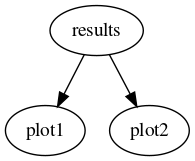
Imagine we want to have two plotting tools plot1 and plot2, each of which takes as an argument the result of the same computation, results, which in turn need a PDF set entered by the user to be computed. One would declare the functions as follows:
def results(pdf):
    #Compute the results
    ...

def plot1(results):
    #Take the result and produce a plot of type 1.
    ...

def plot2(results):
    #Take the result and produce a plot of type 2.
    ...
Then, an input card like the following:
pdf: NNPDF30_nlo_as_0118

actions_:
 - - plot1
   - plot2
Would result in the following DAG:
The important point to note is that parameter names determine the dependencies by default.
To address the inflexibility that results from the way we choose to automatically assign dependency, each action is assigned a unique Namespace specification. This allows to specify actions with several different parameters. Let’s make the example above more complicated:
def results(pdf):
    #Compute the results
    ...

def plot1(results, parameter):
    #Take the result and produce a plot of type 1.
    ...

def plot2(results, parameter):
    #Take the result and produce a plot of type 2.
    ...
We can request a parameter scan like this:
pdf: NNPDF30_nlo_as_0118

scan_params:
  - parameter: 5
  - parameter: 10
  - parameter: 20


actions_:
 - scan_params:
   - plot1
   - plot2
which would result in the following computation:

We have requested the two plots to be computed once in each of the three namespaces spanned by scan_params. The actions are in general not computed in the requested namespace, but rather in the outermost one that satisfies all the dependencies (there is also a unique private stack frame per action not shown in the figures above). That’s why, in the graph above, results appears only once: Since it doesn’t depend on the value of parameter (it doesn’t appear in its signature), it is computed in the root namespace, rather than once in each of the scan_params namespaces. If we instead had this:
pdfs:
 - NNPDF30_nlo_as_0118
 - CT14nlo

scan_params:
  - parameter: 5
  - parameter: 10


actions_:
 - pdfs:
    scan_params:
     - plot1
The corresponding graph would be:
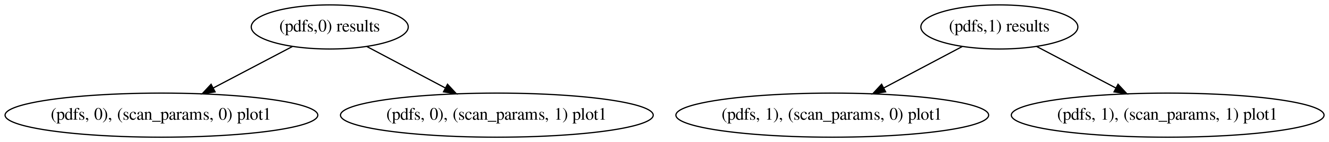
since results does depend on the pdf.
Here we discuss what needs to go from user entered strings in the YAML file plots and reports.
A configuration class derived from reportengine.ConfigParser is used to parse the user input. In validphys, it is defined in validphys.Config.
The parsing in reportengine is context dependent. Because we want to specify resources as much as possible before computing anything (at “compile time”), we need to have some information about other resources (e.g. theory folders) in order to do any meaningful processing.
The Config class takes the user input and the dependencies and:
Returns a valid resource if the user input is valid.
Raises a ConfigError if the user input is invalid.
To parse a given user entered key (e.g. posdataset), simply define a parse_posdataset function. The first argument (i.e. second after self) will be the raw value in the configuration file. Any other arguments correspond to dependencies that are already resolved at the point where they are passed to the function (reportengine takes care of that).
For example, we might have:
def parse_posdataset(self, posset:dict, * ,theoryid):
    ...
The type specification (:dict above) makes sure that the user input is of that type before it is seen by the function (which avoids a bunch of repetitive error checking). A positivity dataset requires a theory ID in order to be meaningfully processed (i.e. to find the folder where the fktables are) and therefore the theoryid will be looked for and processed first.
We need to document what the resource we are providing does. The docstring will be seen in validphys --help config:
def parse_posdataset(self, posset:dict, * ,theoryid):
    """An observable used as positivity constrain in the fit.
    It is a mapping containing 'dataset' and 'poslambda'."""
...In validphys, we use a Loader class to load resources from various folders. It is good to have a common interface, since it is used to list the available resources of a given type or even download a missing resource. The functions of type check_<resource> should take the information processed by the Config class anf verify that a given resources is correct. If so they should return a “Resouce specification” (something typically containing metadata information such as paths, and a load() method to get the C++ object from libnnpdf). We also define a get method that returns the C++ object directly (although I am not sure it’s very useful anymore).
In the case of the positivity set, this is entirely given in terms of existing check functions:
def check_posset(self, theiryID, setname, postlambda):
    cd = self.check_commondata(setname, 0)
    fk = self.check_fktable(theiryID, setname, [])
    th =  self.check_theoryID(theiryID)
    return PositivitySetSpec(cd, fk, postlambda, th)

def get_posset(self, theiryID, setname, postlambda):
    return self.check_posset(theiryID, setname, postlambda).load()
A more complicated example should raise the appropriate loader errors (see the other examples in the class).
The PositivytySetSpec could be defined roughly like:
 class PositivitySetSpec():
     def __init__(self, commondataspec, fkspec, poslambda, thspec):
         self.commondataspec = commondataspec
         self.fkspec = fkspec
         self.poslambda = poslambda
         self.thspec = thspec

     @property
     def name(self):
         return self.commondataspec.name

     def __str__(self):
         return self.name

     @functools.lru_cache()
     def load(self):
         cd = self.commondataspec.load()
         fk = self.fkspec.load()
         return PositivitySet(cd, fk, self.poslambda)
Here PositivitySet is the libnnpdf object. It is generally better to pass around the spec objects because they are lighter and have more information (e.g. the theory in the above example).
With this, our parser method could look like this:
def parse_posdataset(self, posset:dict, * ,theoryid):
    """An observable used as positivity constrain in the fit.
    It is a mapping containing 'dataset' and 'poslambda'."""
    bad_msg = ("posset must be a mapping with a name ('dataset') and "
               "a float multiplier(poslambda)")

    theoryno, theopath = theoryid
    try:
        name = posset['dataset']
        poslambda = float(posset['poslambda'])
    except KeyError as e:
        raise ConfigError(bad_msg, e.args[0], posset.keys()) from e
    except ValueError as e:
        raise ConfigError(bad_msg) from e

    try:
        return self.loader.check_posset(theoryno, name, poslambda)
    except FileNotFoundError as e:
        raise ConfigError(e) from e
The first part makes sure that the user input is of the expected form (a mapping with a string and a number). The ConfigError has support for suggesting that something could be mistyped. The syntax is ConfigError(message, bad_key, available_keys). For example, if the user enters “poslanda” instead of “postlambda”, the error message would suggest the correct key.
Note that all possible error paths must end by raising a ConfigError.
It is possible to easily process list of elements once the parsing for a single element has been defined. Simply add an eleement_of decorator to the parsing function:
@element_of('posdatasets')
def parse_posdataset(self, posset:dict, * ,theoryid):
Now posdatasets is parsed as a list of positivity datasets, and can be used to loop over in namespace specifications.
Now that we can receive positivity sets as input, let’s do something with them. The SWIG wrappers allow us to call the C++ methods of libnnpdf from Python. These things go in the validphys.results module. We can start by defining a class to produce and hold the results:
class PositivityResult(StatsResult):
    @classmethod
    def from_convolution(cls, pdf, posset):
        loaded_pdf = pdf.load()
        loaded_pos = posset.load()
        data = loaded_pos.GetPredictions(loaded_pdf)
        stats = pdf.stats_class(data.T)
        return cls(stats)

    @property
    def rawdata(self):
        return self.stats.data
pdf.stats_class allows to interpret the results of the convolution as a function of the PDF error type (e.g. to use the different formulas for the uncertainty of Hessian and Monte Carlo sets).
And then define a simple provider function:
def positivity_predictions(pdf, positivityset):
return PositivityResult.from_convolution(pdf, positivityset)In the user interface we have the possibility to perform a computation looping over a list of namespaces. In the code, we can define providers that collect the results of such computations with the collect function.
The signature is:
collect(function, fuzzyspec)This will expand the fuzzyspec relative to the current namespace and compute the function once for each frame. Then it will put all the results in a list (to be iterated in the same order as the fuzzyspec) and set that as the result of the provider.
For example
possets_predictionsa = collect(positivity_predictions, ('posdatasets',))Compared to a simple for loop, the collect function has the advantages that the computations are appropriately reused and several results could be computed simultaneously in the parallel mode.
We can use the output of collect as input to other providers. For example:
def count_negative_points(possets_predictions):
    return np.sum([(r.rawdata < 0).sum(axis=1) for r in
possets_predictions], axis=0)Providers can checks that verify that all the required preconditions are met. Checks are executed at the time at which the call node is just created and all its required dependencies are either in the namespace or scheduled to be produced. Checking functions take the current state of the namespace, as well as an unspecified set of other parameters (because I haven’t decided on the interface yet!). Therefore check functions should accept **kwargs arguments. Checks are decorated with the reportengine.checks.make_argcheck function. If checks don’t pass, they must raise a reportengine.checks.CheckError exception.
For example, given a reweighting function, we may want to check that the current PDF (the value that will be passed to the function) has a Monte Carlo error type, we might define a check like:
@make_check
def check_pdf_is_montecarlo(ns, **kwargs):
    pdf = ns['pdf']
    etype = pdf.ErrorType
    if etype != 'replicas':
        raise CheckError("Error type of PDF %s must be 'replicas' and not %s"
                          % (pdf, etype))
Checks can be used (abused) to modify the namespace before the action function sees it. This can be used for some advanced context dependent argument default setting (for example setting default file names based on the nsspec).
The check is associated to the provider function by simply applying it as a decorator:
@check_pdf_is_montecarlo
def chi2_data_for_reweighting_experiments(pdf, args):
    ...
A slightly higher level interface to checks is implemented by the make_argcheck decorator. Instead of receiving a namespace and other unspecified arguments, like the functions decorated with make_check, it simply takes the arguments we want to test. The function can return a dictionary that will be used to update the namespace (but that is not required, it can also not return anything).
For example the check_pdf_is_montecarlo above could be more easily implemented like:
@make_argcheck
def check_pdf_is_montecarlo(pdf):
    etype = pdf.ErrorType
    if etype != 'replicas':
        raise CheckError("Error type of PDF %s must be 'replicas' and not %s"
                          % (pdf, etype))
make_argcheck should be preferred, since it is more explicit, and could be extended with more functionality later on. However it is newer and not very used currently in the code.
Checks have no effect outside of reportengine (unless you call them explicitly).
Ideally, the checks should be sufficient to guarantee that the actions will not fail at runtime.
In order to produce figures, just decorate your functions returning matplotlib Figure objects with the reportengine.figure.figure function, e.g.:
@figure
def plot_p_alpha(p_alpha_study):
   fig, ax = plt.subplots()
   #Plot something
   ...
   return fig
This will take care of the following:
Saving the figures with a nice, unique name to the output folder, in the formats specified by the user.
Closing the figures to save memory.
Making sure figures are properly displayed in reports.
There is also the figuregen decorator for providers that are implemented as generators that yield several figures (see e.g. the implementation of plot_fancy). Apart from just the figure, yield a tuple (prefix, figure) where the prefix will be used in the filename.
These work similarly to figures, as described above. Instead use the @table and @tablegen decorators.
Tables will be saved in the CSV formats.
By default, the str() method will be applied to objects that appear in the report. If you want a custom behaviour, declare a declare a custom as_markdown property for your objects. It should return a string in Pandoc Markdown describing your object. Raw HTML is also allowed (although that decreases the compatibility, e.g. if we decide to output LaTeX instead of HTML in the future).