Introduction
The immediate aim of validphys2 is to serve as a both very agile and highly reliable analysis framework for NNPDF, but the goal extends beyond. When the time comes, this framework should become the common gateway that all the NNPDF code uses, providing features ranging from from automated report generation to automatic detection of problems with the fits.
The project is separated in two codes with well defined and separated scopes:
- reportengine
- It is a compiler of user-entered configuration (in the YAML format) into directed acyclic graphs of Python executable functions, which are defined by client applications. One such function that comes with
reportengineisreport, which processes a template in the Markdown format, with special tags that signify the resources requested by the user, and produces an HTML report (See Reports). Apart from the compiler functionality,reportenginealso provides general application utilities such as crash handlers and a help system. - validphys2
- It is a set of higher level tools operating on the NNPDF resources, which can be used either within a
reportengineapplication or standalone. It is based on thelibnnpdfPython wrappers, and extends them with extra functionality (related to error checking, loading and downloading among others). The NNPDF objects are then used in functions producing plots, tables and other outputs (such as reweighted PDF sets).
What is working
Right now the following features are implemented:
- Processing of libnnpdf resources.
- Data-Theory plotting specification.
- PDF comparisons.
- A framework for fitting parameters such as αS bases on series of fits.
- Plots and tables showing statistical estimators.
- Generation of reweighted sets.
- Report generation from templates.
- Automatic downloading of PDFs, fits and theories.
- Automatic uploading of reports and other outputs.
- Standalone executables implementing functionality such as
postfitor uploading and downloading resources.
These features are documented in more detail in Usage.
Design considerations
Look before you leap
A scientific program usually requires a large set of complex input parameters and can take a very long time to produce results. Results tend to be frequently unexpected even if everything is working correctly. It is essential to check that the inputs are correct and make sense. Thus good error reporting capabilities are an important design consideration.
Also, the inputs of a given function should be checked as early as possible, which is not necessarily at the point of the program where the function is to be called. For example, something like this:
def check_parameter_is_correct(parameter):
    ...

def plot(complex_calculation, parameter):
    check_parameter_is_correct(parameter)
    #make plot
    ...
has the disadvantage that in order to get to the check, we presumably need to compute complex_calculation first, and that could be a waste of time if it turns out that parameter is not correct for some reason and we can’t do the plot anyway. Instead we should arrange to call check_parameter_is_correct(parameter) as early as possible (outside the plotting function) and show the user an informative error message.
All inputs should be checked as early as possible. If the checks pass, the program should not fail.
Of course it is impossible to guarantee that this is always going to happen. For example it is possible that we check that a folder exists and we have permissions to write to it, but by the time we actually need to write, the folder has been deleted. However in such cases the state of the program can be considered broken and it’s OK to make it fail completely.
There is an API for early checks in reportengine. We would write something like:
@make_argcheck
def check_parameter_is_correct(parameter):
    ...

@check_parameter_is_correct
def plot(complex_calculation, parameter):
    #make plot
    ...
The checking function will now be called as soon as the program realizes that the plot function will be required eventually (at “compile time”). The user would be shown immediately an error message explaining why the parameter is wrong.
The fancy term for this style of coding is Contract Programming.
Declarative input
It is extremely convenient to be able to specify the what the program should only without any regard of knowledge of how that is achieved by the underlying implementation. The current nnfit input files are a good example of this. The primary input of validphys are YAML run cards. A very simple one looks like this:
pdfs:
    - NNPDF30_nlo_as_0118
    - NNPDF30_nnlo_as_0118
    - CT14nlo

norm:
    normalize_to: NNPDF30_nlo_as_0118

first:
    Q: 1
    flavours: [up, down, gluon]

second:
    Q: 100
    xgrid: linear

actions_:
    - first::norm plot_pdfreplicas
    - first plot_pdfs
- second plot_pdfreplicas- Correct by definition
A declarative input specifies what you want. It is up to the underlying code to try to provide it (or fail with an informative message).
- Obvious meaning
It is easy for a human to verify that the input is indeed what it was intended. Even without any explanation it should be easy enough to guess what the runcard above does.
- Implementation independent
The input is very loosely coupled with the underlying implementation, and therefore it is likely to remain valid even after big changes in the code are made. For example, in the runcard above, we didn’t have to concern ourselves with how LHAPDF grids are loaded, and how the values of the PDFs are reused to produce the different plots. Therefore the underlying mechanism could change easily without breaking the runcard.
Therefore:
- The primary input mechanism should be an easy to read input with an obvious meaning and independent of implementation details.
Usage as a programmatic API
While the goal of reportengine is to allow simple and easily repeatable bach actions, sometimes it is far simpler to get the work done with a raw (Python) script, or it is needed to explore the outcomes using something like an Jupyter notebook. It would be good to be able to use all the tools that already exist in validphys for that, without needing to reinvent the wheel or to alter functions so that for example they don’t write data to some preconfigured path. Therefore:
- The various computing and plotting tools should work well when included in a normal script that doesn’t use the reportengine graph compiler.
This is implemented by making sure that as much as possible all the validphys functions are pure. That is, the output is a deterministic function of the inputs, and the function has no side effects (e.g. no global state of the program is altered, nothing is written to disk). There are some exceptions to this though. For example the function that produces a reweighted PDF set needs to write the result to disk. The paths and side effects for other more common results like figures are managed by reportengine. For example, the @figure decorator applied to a function that returns a Python (matplotlib) figure will make sure that the figure is saved in the output path, with a nice filename, while having no effect at all outside the reportengine loop. The same goes for the check functions described above.
Easy to loop
Very frequently there is the need to compare. It is easy enough to write simple scripts that loop over the required configurations, but that cannot scale well when requirements change rapidly (and is also easy to make trivial mistakes). Therefore reportengine allows configurations to easily loop over different sets of inputs. For example the following runcard:
pdfs:
    - id:  160502-r82cacd2-jr-001
      label: Baseline

    - id: 160502-r82cacd2-jr-008
      label: HERA+LHCb

    - id: 160603-r654e559-jr-003
      label: baseline+LHCb and Tev legacy

fit: 160603-r654e559-jr-003
theoryids:
    - 52
    - 53
use_cuts : nocuts

experiments:
  - experiment: LHCb
    datasets:
      - { dataset: LHCBWZMU7TEV, cfac: [NRM] }
      - { dataset: LHCBWZMU8TEV, cfac: [NRM] }

  - experiment: ATLAS
    datasets:
      - { dataset: ATLASWZRAP36PB}

actions_:
 - theoryids::pdfs::experiments::experiment plot_fancy
Will produce a separate plot for each combination of the two theories (52 and 53), the three pdfs at the top, and each dataset in the two experiments (so 18 plots in total). This syntax is discussed in more detail in the Usage section.
- It should be trivial to repeat an action for different sets of inputs.
Lazy processing
The requirements above (in particular the combination of early checking and arbitrary looping) lead to the condition that the value of the resources depends on the other resources involved. For example, a dataset requires a theoryid in order to locate the FKTables and cfactors, and we want to check that these paths exist early on.
Therefore the processing always starts from the user requirement (i.e. the requested actions) and processes each requirement for that action within the correct context, trying to avoid duplicating work. Conversely we ignore everything that is not required to process the actions.
Usage
Installing
A lot of work has gone into producing a usable installer that works on both Linux and Mac. Currently the installation for both platforms boils down to executing a script.
Producing installers is a difficult (and boring) problem since a lot of dependencies need to be set up to work properly together. In practice, it is hard to produce a set of instructions that work reliably on all platforms and with all compilers. This is further complicated by the fact that the Python deployment tools are substandard in several ways (such as avoiding unwanted interaction between libraries for Python 2 and Python 3). Furthermore, on Mac gcc and clang interact poorly when it comes to including the C++ standard library, and a lot of care has to be taken to include the correct one.
The solution to all that is to provide precompiled versions of all the dependencies, that are generated automatically when new commits are pushed to the CERN Gitlab server (for Linux) and the Travis CI server (for Mac).
The compiled binaries are subsequently packaged (using conda) and uploaded to a remote server where they are accessible. These packages are known to compile on clean default environments (namely those of the CI servers used to produce the packages), and the Python packages are known to be importable. Everything that an user has to do is to configure conda correctly and ask it to install the nnpdf. This results in an environment that contains not only an usable version of validphys, but also of the nnpdf code and all its dependencies (including for example LHAPDF and APFEL). Therefore an user who doesn’t need to modify the code should not need to compile anything to work with the NNPDF related programs. This should be useful in clusters where we don’t completely control the environment and frequently need to deal with outdated compilers.
Installation steps
A helper script exists to aid the configuration. All you need to do is:
#Obtain the helper script
git clone git@github.com:NNPDF/binary-bootstrap.git
#Execute the script
./binary-bootstrap/bootstrap.sh
The script will ask for the password of the NNPDF private repositories. You can find it here:
https://www.wiki.ed.ac.uk/pages/viewpage.action?spaceKey=nnpdfwiki&title=Git+repository+instructions
The conda installer will ask to add the conda bin path to the default $PATH environment variable (by editing your .bashrc file). Confirm this unless you know that you have a specific reason not to. Note that newer versions of conda give the option of having conda available, but not any environment (which you have to enable explicitly by either having conda activate in .bashrc or typing it each time you want to use the environment). On remote machines, the addition to .bashrc should read as follows:
the if condition is important because conda activate prints to the standard output, which interferes with commands like scp and rsync.
Not that the script may ask you to perform some actions manually ( e.g. it will not overwrite your existing conda configuration). Please pay attention to the output text of the script.
Once everything is configured, you can install the code running:
conda install nnpdfThis will provide functioning C++ and Python executables.
Linking existing LHAPDF grids
The installer will set up it’s own version of the LHAPDF code, with its own path for storing PDFs, which can be seen running lhapdf --help. If you have an exiting folder with LHAPDF grids, you may want to either move, symlink or copy them to the new path (depending on whether you want to keep around the older installation). The command for symlinking would be something like:
ln -s <old path>/share/LHAPDF/* <new path>/miniconda3/share/LHAPDFThis will avoid symlinking the existing LHAPDF configuration, which may be corrupted or incompatible. You should make sure only the grid folders are transferred if you copy or move instead.
Troubleshooting
After several iterations on the install system most issues have been resolved. There could be problems derived from interactions with hacks targeted at solving environment problems manually. In particular, see that you don’t have any PYTHONPATH environment variable (for example pointing at some version of LHAPDF) since that will overwrite the default conda configuration. This is easily solved by removing said hacks from .bashrc or similar files.
A different source of problems is the priority order of the conda channels: We use dependency packages from the official Anaconda defaults channel, as well as from the community conda-forge channel. If a package exists in both channels, the one from the channel declared first .condarc file is the one that gets selected. Unfortunately the packages are not always binary compatible and therefore the wrong priority causes various sorts of compiler errors. Also unfortunately, what the wrong priority is changes over time, depending on the features that both channels provide. Currently we use the compilers from the defaults channel, and therefore it has to be declared first.
If you include conda in your default PATH, the default Python version will be the conda Python 3. This could cause problems if you use code that expects /usr/bin/env python to point to Python 2. In such cases you will need to conditionally enable or disable conda. You can save a helper executable script (called for example use-conda) to some location in your PATH containing:
Remember to chmod +x use-conda. Now typing:
source use-condawill set your PATH environment variable to point to the conda binaries.
In any case this tends to not be a problem for newer software as Python 3 gains support.
Development installs
Installing the nnpdf conda package is sufficient for running the NNPDF tools. In addition it is possible to set up a development environment in a way that it can be modified and then rebuilt. In general, you can install all the runtime dependencies of a package (like) nnpdf with conda install <package> --only-deps. Note that you still need to obtain the build dependencies.
The development environment as described here works for developing the NNPDF code. Other external projects might work within the development environment in a similar way, but configuring them may prove more difficult (for example due to build scripts with hard coded paths). Thus contributing conda recipes for those is highly encouraged when they can be generally useful.
Setting up a C++ development environment
The easiest way to work with C++ code that depends on nnpdf or other C++ packages (or indeed to develop nnpdf itself) is to set up a development conda environment. While the existing packages should run on any relevant Linux or Mac system, linking to them is a different matter: The most straightforward way of doing so is using the same compiler toolchain that was used to generate the packages. You may find some relevant documentation here. You need to create a conda environment that has the required dependencies of your project, including the relevant build toolchain (including things like a C++ compiler). For example here is how we would set up a development environment for nnpdf.
Find out the C++ (or C or FORTRAN) compiler package name for your platform here. For example, the C++ compilers for Linux and macOS are
gxx_linux-64andclangxx_osx-64respectively.Create an environment with all the build and runtime dependencies. We start off with:
$ conda create -n nnpdf-dev
#Install the runtime dependencies of nnpdf
$ conda install --only-deps nnpdf
#Install the c++ compiler for Linux (see above)
$ conda install gxx_linux-64
Note that when the environment is activated, many environment variables pointing to the compiler paths are activated for us:
$ source activate nnpdf-dev
INFO: activate-binutils_linux-64.sh made the following
environmental changes:
+ADDR2LINE=/home/zah/anaconda3/envs/nnpdf-dev/bin/x86_64-conda_cos6-linux-gnu-addr2line
+AR=/home/zah/anaconda3/envs/nnpdf-dev/bin/x86_64-conda_cos6-linux-gnu-ar
+AS=/home/zah/anaconda3/envs/nnpdf-dev/bin/x86_64-conda_cos6-linux-gnu-as
+CXXFILT=/home/zah/anaconda3/envs/nnpdf-dev/bin/x86_64-conda_cos6-linux-gnu-c++filt
+ELFEDIT=/home/zah/anaconda3/envs/nnpdf-dev/bin/x86_64-conda_cos6-linux-gnu-elfedit
+GPROF=/home/zah/anaconda3/envs/nnpdf-dev/bin/x86_64-conda_cos6-linux-gnu-gprof
+HOST=x86_64-conda_cos6-linux-gnu
+LD_GOLD=/home/zah/anaconda3/envs/nnpdf-dev/bin/x86_64-conda_cos6-linux-gnu-ld.gold
+LD=/home/zah/anaconda3/envs/nnpdf-dev/bin/x86_64-conda_cos6-linux-gnu-ld
+NM=/home/zah/anaconda3/envs/nnpdf-dev/bin/x86_64-conda_cos6-linux-gnu-nm
+OBJCOPY=/home/zah/anaconda3/envs/nnpdf-dev/bin/x86_64-conda_cos6-linux-gnu-objcopy
+OBJDUMP=/home/zah/anaconda3/envs/nnpdf-dev/bin/x86_64-conda_cos6-linux-gnu-objdump
+RANLIB=/home/zah/anaconda3/envs/nnpdf-dev/bin/x86_64-conda_cos6-linux-gnu-ranlib
+READELF=/home/zah/anaconda3/envs/nnpdf-dev/bin/x86_64-conda_cos6-linux-gnu-readelf
+SIZE=/home/zah/anaconda3/envs/nnpdf-dev/bin/x86_64-conda_cos6-linux-gnu-size
+STRINGS=/home/zah/anaconda3/envs/nnpdf-dev/bin/x86_64-conda_cos6-linux-gnu-strings
+STRIP=/home/zah/anaconda3/envs/nnpdf-dev/bin/x86_64-conda_cos6-linux-gnu-strip
INFO: activate-gcc_linux-64.sh made the following environmental
changes:
+CC=/home/zah/anaconda3/envs/nnpdf-dev/bin/x86_64-conda_cos6-linux-gnu-cc
+CFLAGS=-march=nocona -mtune=haswell -ftree-vectorize -fPIC
-fstack-protector-strong -fno-plt -O2 -pipe
+CPPFLAGS=-D_FORTIFY_SOURCE=2 -O2
+CPP=/home/zah/anaconda3/envs/nnpdf-dev/bin/x86_64-conda_cos6-linux-gnu-cpp
+DEBUG_CFLAGS=-march=nocona -mtune=haswell -ftree-vectorize -fPIC
-fstack-protector-strong -fno-plt -O2 -pipe -Og -g -Wall -Wextra
-fcheck=all -fbacktrace -fimplicit-none -fvar-tracking-assignments
+GCC_AR=/home/zah/anaconda3/envs/nnpdf-dev/bin/x86_64-conda_cos6-linux-gnu-gcc-ar
+GCC=/home/zah/anaconda3/envs/nnpdf-dev/bin/x86_64-conda_cos6-linux-gnu-gcc
+GCC_NM=/home/zah/anaconda3/envs/nnpdf-dev/bin/x86_64-conda_cos6-linux-gnu-gcc-nm
+GCC_RANLIB=/home/zah/anaconda3/envs/nnpdf-dev/bin/x86_64-conda_cos6-linux-gnu-gcc-ranlib
+LDFLAGS=-Wl,-O2 -Wl,--sort-common -Wl,--as-needed -Wl,-z,relro
-Wl,-z,now
+_PYTHON_SYSCONFIGDATA_NAME=_sysconfigdata_x86_64_conda_cos6_linux_gnu
INFO: activate-gxx_linux-64.sh made the following environmental
changes:
+CXXFLAGS=-fvisibility-inlines-hidden -std=c++17
-fmessage-length=0 -march=nocona -mtune=haswell -ftree-vectorize
-fPIC -fstack-protector-strong -fno-plt -O2 -pipe
+CXX=/home/zah/anaconda3/envs/nnpdf-dev/bin/x86_64-conda_cos6-linux-gnu-c++
+DEBUG_CXXFLAGS=-fvisibility-inlines-hidden -std=c++17
-fmessage-length=0 -march=nocona -mtune=haswell -ftree-vectorize
-fPIC -fstack-protector-strong -fno-plt -O2 -pipe -Og -g -Wall
-Wextra -fcheck=all -fbacktrace -fimplicit-none
-fvar-tracking-assignments
+GXX=/home/zah/anaconda3/envs/nnpdf-dev/bin/x86_64-conda_cos6-linux-gnu-g++
These environment variables are read and interpreted by build systems such as
cmake, so that building a project normally will use the conda compilers, when the build system has been configured with this environment. Note that forcmakethis means that the environment has to be activated at the moment you run thecmakeexecutable.Obtain the dependencies of the code you want to build. Where to find those depends on the particular cod. For example, something linking to
libnnpdfwill likely requirepkg-config. Projects based onautotools(those that have a./configurescript) will additionally requireautomakeandlibtool. Similarly projects based oncmakewill require installing thecmakepackage. In the case ofnnpdfitself, the build dependencies can be found in<nnodf git root>/conda-recipe/meta.yaml. We have to install the remaining ones manually:$ conda install pkg-config swig=3.0.10 cmakeWhere we also installed the C++ compiler in the previous step.
Note that you should not have the
nnpdfpackage installed in the conda environment used for development. You can remove it withconda remove nnpdf.Build the project: Assuming the environment is set, the only remaining requirement is setting the installation prefix to point to the
condaenvironment. This is conveniently stored in the$CONDA_PREFIXenvironment variable. We would build the nnpdf project like this:nnpdf$ mkdir conda-bld nnpdf$ cd conda-bld #We have something like $CONDA_PREFIX==~/anaconda3/envs/nnpdf-dev/ nnpdf/conda-bld$ cmake .. -DCMAKE_INSTALL_PREFIX=$CONDA_PREFIXNote that you need to execute this while the environment created above is activated. Both the compilers and all dependencies are now found inside the environment. The output of the
cmakecommand above is:-- Setting build type to 'Release' as none was specified. -- The C compiler identification is GNU 7.2.0 -- The CXX compiler identification is GNU 7.2.0 -- Check for working C compiler: /home/zah/anaconda3/envs/nnpdf-dev/bin/x86_64-conda_cos6-linux-gnu-cc -- Check for working C compiler: /home/zah/anaconda3/envs/nnpdf-dev/bin/x86_64-conda_cos6-linux-gnu-cc -- works -- Detecting C compiler ABI info -- Detecting C compiler ABI info - done -- Detecting C compile features -- Detecting C compile features - done -- Check for working CXX compiler: /home/zah/anaconda3/envs/nnpdf-dev/bin/x86_64-conda_cos6-linux-gnu-c++ -- Check for working CXX compiler: /home/zah/anaconda3/envs/nnpdf-dev/bin/x86_64-conda_cos6-linux-gnu-c++ -- works -- Detecting CXX compiler ABI info -- Detecting CXX compiler ABI info - done -- Detecting CXX compile features -- Detecting CXX compile features - done -- Found PkgConfig: /home/zah/anaconda3/envs/nnpdf-dev/bin/pkg-config (found version "0.29.2") -- Checking for one of the modules 'libarchive' -- Checking for one of the modules 'sqlite3' -- Checking for one of the modules 'gsl' -- Checking for one of the modules 'yaml-cpp' -- Configuring done -- Generating done -- Build files have been written to: /home/zah/nngit/libnnpdf/conda-bldWe can now proceed normally:
$ make
$ make install
This should result in a working installation, both for the C++ and Python parts of the code.
Use the result. For example, we can now compile
buildmasterlinking with thelibnnpdflibrary we just created. Since the conda environment is all set andbuildmasterinstalls in a fixed location by default, no additional configuration is necessary:buildmaster$ mkdir bld && cd bld buildmaster/bld$ cmake .. buildmaster/bld$ make -j && make install
Developing Python projects
Python code should be installed in the specific folder of the conda environment. This is handled automatically when the environment is activated. Like with C++ projects we need to make sure to have the correct dependencies in our environment, and that varies by project.
In addition since we do not need to compile Python we would like that the changes we make to the code are reflected automatically when we run it. To that end, we can run the following command for projects containing a setup.py file.
pip install --ignore-installed -e .This command will symlink the relevant files to our conda prefix and allow the modules to me imported from the conda version of python. Note that the validphys2 works like this by default when you install the nnpdf project with make install, and so does not require any additional configuration.
Updating
In most cases running conda update <package> will do the right thing, and update the package with the requested dependencies.
If you are interested in a specific version (not necessarily the latest one), you can run conda install <package>=<version>.
Note that, in case you are doing Development installs, the process is somewhat more manual, and you might need to update each dependency of the package you are developing. A convenient shortcut might be to install the desired version of the development package with conda, so it takes care of the dependencies, and the conda version and setting up the development version again.
Seeing what actions are available
A help command is generated automatically by reportengine. The command
will show you the modules that contain the actions (as well as the usual description of the command line flags). For example,
will list all the actions defined in the plots module together with a brief description of each of them. Asking for the help of one of the actions, like for example:
will list all the inputs that are required for this action. For example the command below results currently in the following output:
plot_fancy

Defined in: validphys.dataplots

Generates: figuregen

plot_fancy(one_or_more_results, commondata, cuts, normalize_to:
  (<class 'int'>, <class 'str'>, <class 'NoneType'>) = None)

Read the PLOTTING configuration for the dataset and generate the
corrspondig data theory plot.

The input results are assumed to be such that the first one is the
data, and the subsequent ones are the predictions for the PDFfs. See
``one_or_more_results``. The labelling of the predictions can be
influenced by setting ``label`` attribute of theories and pdfs.

normalize_to: should be either 'data', a pdf id or an index of the
result (0 for the data, and i for the ith pdf). None means plotting
absolute values.

See docs/plotting_format.md for details on the format of the PLOTTING
files.

The following resources are read from the configuration:

    dataset_input: The mapping that corresponds to the dataset
  specifications in the fit files
  [Used by commondata]

    theoryid: A number corresponding to the database theory ID where
  the corresponding theory folder is installed in te data directory.
  Either just an id (str or int), or a mapping with 'id' and 'label'.
  [Used by cuts]

    use_cuts(bool or str): Whether to filter the points based on the
  cuts applied in the fit, or the whole data in the dataset. The
  possible options are:

  - internal: Calculate the cuts based on the existing rules. This
  is
    the default.

  - fromfit: Read the cuts stored in the fit.

  - nocuts: Use the whole dataset.
  [Used by cuts]

    fit: A fit in the results folder, containing at least a valid
  filter result. Either just an id (str), or a mapping with 'id' and
  'label'.
  [Used by commondata]

    use_fitcommondata(bool): Use the commondata files in the fit
  instead of those in the data directory.
  [Used by commondata]

    pdfs(list): A list of pdf objects.
  [Used by one_or_more_results]

    pdf: A PDF set installed in LHAPDF. Either just an id (str), or a
  mapping with 'id' and 'label'.
  [Used by one_or_more_results]

    use_t0(bool): Whether to use the t0 PDF set to generate
  covariance matrices.
  [Used by t0set]

    t0pdfset: PDF set used to generate the t0 covmat.
  [Used by t0set]

The following additionl arguments can be used to control the
behaviour. They are set by default to sensible values:

  normalize_to(int or str or NoneType) = None
  q2min(Number or NoneType) = None [Used by cuts]
  w2min(Number or NoneType) = None [Used by cuts]
  check_plotting(bool) = False [Used by dataset]
We can see which keys have a special meaning in the configuration file with:
All other keys are interpreted literally (although they could be further processed by specific actions).
Writing input cards
Input cards are YAML files that describe the input resources, together with the actions we want to perform on them.
Let’s begin with a simple example:
pdf: NNPDF30_nlo_as_0118

theoryid: 52

use_cuts: "nocuts"

dataset_input:
    dataset: ATLASWZRAP36PB
    cfac: [EWK]

actions_:
  - plot_fancy
  - plot_chi2dist
We are specifying one PDF (by the LHAPDF id), one dataset and one theory. Note that the dataset specification is identical to that of the nnfit configuration files.
We are saying that we do not want to use the cuts of the data (so we don’t have to specify a fit containing the cut data).
The special actions_ key is used to declare the actions we want to have executed. The syntax is the same as for the targets inside the report, and discussed in detail in the Report template specification. We want a data/theory comparison (plot_fancy) and to plot the distribution of the chi² for each replica (plot_chi2dist). If we save the above runcard to a file called runcard.yaml we can produce the plots with:
Multiple inputs and namespaces
Resources can be declared at top level, like in the example above, inside a mapping (with an arbitrary key), or inside an element of a list of mappings.
Arbitrary namespaces
For example, we can modify the example as follows:
pdf: NNPDF30_nlo_as_0118

theoryid: 52

fit: 161222-jr-004

with_cuts:
  use_cuts: "fromfit"

without_cuts:
  use_cuts: "nocuts"

dataset_input:
    dataset: ATLASWZRAP36PB
    cfac: [EWK]

actions_:
  - with_cuts plot_fancy
  - without_cuts plot_chi2dist
Here with_cuts and without_cuts are arbitrary strings that specify namespaces. Now we are asking for one action (plot_fancy) to be executed taking into account the cuts (note that we have also specified the fit where we read them from) and another (plot_chi2dist) to be executed without the cuts. Similar to a programming language like C, the inner namespaces has priority with respect to the outer. For example if we add a PDF specification to the “with_cuts” namespace like this:
pdf: NNPDF30_nlo_as_0118

theoryid: 52

fit: 161222-jr-004

with_cuts:
  use_cuts: "fromfit"
  pdf: CT14nlo

without_cuts:
  use_cuts: "nocuts"

dataset_input:
    dataset: ATLASWZRAP36PB
    cfac: [EWK]

actions_:
  - with_cuts plot_fancy

  - without_cuts plot_chi2dist
The plot_fancy action will ignore the outer pdf (NNPDF30_nlo_as_0118) and use the one defined in the innermost namespace (CT14nlo). Because we have not specified plot_chi2dist to be executed within the with_cuts namespace, it will continue to use NNPDF.
Lists of namespaces
We can also have lists of mapping acting as namespaces. The action will then be repeated inside each of the namespaces generating one result for each. For example:
pdf: NNPDF30_nlo_as_0118

theoryid: 52

fit: 161222-jr-004

specifications:
- use_cuts: "fromfit"
  pdf: CT14nlo

- use_cuts: "nocuts"

dataset_input:
    dataset: ATLASWZRAP36PB
    cfac: [EWK]

actions_:
  - specifications plot_fancy
Now a different plot_fancy action will be executed for each of the two mappings of the list “specifications”: One will use the CT PDF and use the cuts, and the other will plot all points in the dataset.
Some keys are appropriately interpreted either as lists of objects or list or namespaces depending on the context. They are documented in validphys --help config. For example, the pdfs key is entered as a list of LHAPDF ids:
Because the plot_fancy action takes a list of pdfs as input, something like this:
pdfs:
  - NNPDF30_nlo_as_0118
  - CT14nlo
theoryid: 52
use_cuts: "nocuts"
dataset_input:
dataset: ATLASWZRAP36PB
cfac: [EWK]
actions_:
- plot_fancywill produce plots where the two pdfs appear together. However we can also produce individual plots for each pdf, by simply specifying that we want to loop over the pdfs:
pdfs:
  - NNPDF30_nlo_as_0118
  - CT14nlo

theoryid: 52

use_cuts: "nocuts"

dataset_input:
    dataset: ATLASWZRAP36PB
    cfac: [EWK]

actions_:
  - pdfs plot_fancy
In this case the value of the pdfs key is seen as equivalent to:
However the special treatment allows us to simplify both the input file and the programmatic interface of the functions (see [Automatic Lists]).
Nesting namespaces
Namespace specifications like those described above can be arbitrarily nested. Values will be searched from inner to outer namespace. When the namespace specifications represent lists of mappings, all possible combinations will be produced.
Consider the example:
pdfs:
    - 160502-r82cacd2-jr-001

    - 160502-r82cacd2-jr-008

    - 160603-r654e559-jr-003

fit: 160603-r654e559-jr-003
theoryids:
    - 52
    - 53

with_cuts:
    use_cuts : "nocuts"

experiments:
  - experiment: LHCb
    datasets:
      - { dataset: LHCBWZMU7TEV, cfac: [NRM] }
      - { dataset: LHCBWZMU8TEV, cfac: [NRM] }

  - experiment: ATLAS
    datasets:
      - { dataset: ATLASWZRAP36PB}

actions_:
  - with_cuts::theoryids::pdfs::experiments::experiment plot_fancy
This will first enter the “with_cuts” namespace (thus setting use_cuts="nocuts" for the action), and then loop over all the theories, pdfs, experiments and datasets inside each experiment (note that when used as a namespace specification, experiment refers to the list of datasets it contains).
The order over which the looping is done is significative: For one the outer specifications must set all the variables required for the inner to be fully resolved (so with_cuts must go before experiment).
For other, the caching mechanism works by grouping together the namespace specifications from the beginning. For example, suppose we where to add another action to the example above:
both of these require to compute the same convolutions. Validphys will realize this as long as both actions are iterated in the same way. However permuting “pdfs” and “theoryids” would result in the convolutions computed twice, since the code cannot prove that they would be identical.
Always loop from more general to more specific.
Always loop in the same way.
Action arguments
Action arguments are syntactic sugar for specifying arguments visible to a single actions. They are subject to being verified by the action defined checks. For example, in the PDF plotting example above:
pdfs:
    - NNPDF30_nlo_as_0118
    - NNPDF30_nnlo_as_0118
    - CT14nlo

first:
    Q: 1
    flavours: [up, down, gluon]

second:
    Q: 100
    xgrid: linear

actions_:
  - first::plot_pdfreplicas (normalize_to=NNPDF30_nlo_as_0118)
  - first plot_pdfs
  - second plot_pdfreplicas
The normalize_to key only affects the plot_pdfreplicas action. Note that defining it inside the first mapping would have had the same effect in this case.
The from_ special key
The from_ specifies that the value of a resource is to be taken from a container. This is useful for working with fits (but not limited to that). For example:
fit: 161208-jr-003

use_cuts: "nocuts"

description:
    from_: fit

theory:
    from_: fit

theoryid:
    from_: theory


Q: 10

template: report.md

normalize:
    normalize_to: 1

datanorm:
    normalize_to: data

pdfs:
    - from_: fit
    - NNPDF30_nlo_as_0118
experiments:
    from_: fit

actions_:
   - report(out_filename=index.md)
Here the from_ key is used multiple times:
To obtain the description string from the report input card.
To obtain the theory mapping from the fit input card.
To obtain the theoryid key from the theory mapping.
To obtain a single PDF produced in the fit (as an element of the list/namespaces of pdfs). Note that the keyword is also allowed inside nested elements.
To obtain a set of all the experiments of the fit.
The from_ key respects lazy processing, and therefore something like this will do what you expect:
fits:
    - 161208-jr-003
    - 161222-jr-004


use_cuts: "nocuts"

theory:
    from_: fit

theoryid:
    from_: theory


Q: 10

description:
    from_: fit
template: report.md

normalize:
    normalize_to: 1

datanorm:
    normalize_to: data

pdfs:
    - from_: fit
    - NNPDF30_nlo_as_0118
experiments:
    from_: fit

actions_:
  - fits report
This will work exactly as the example above, except that a new action (with its corresponding different set of resources) will be generated for each of the two fits.
For fits, there is a shortcut to set experiments, pdf and theoryid to the values obtained from the fit. This can be done with the fitcontext rule. The above example can be simplified like this:
fits:
    - 161208-jr-003
    - 161222-jr-004


use_cuts: "nocuts"


Q: 10

description:
    from_: fit
template: report.md

normalize:
    normalize_to: 1

datanorm:
    normalize_to: data

pdfs:
    - from_: fit
    - NNPDF30_nlo_as_0118

actions_:
  - fits::fitcontext report
Note that one still needs to set manually other keys like description and pdfs.
from_: Null
As a special case, from_: Null will retrieve the variable from the current namespace. This comes handy to transform lists of items into other items. Consider for example:
base:
    fit: NNPDF31_nnlo_as_0118_1000


pairs:
    fits:
        - from_: base
        - from_: null

fits:
    - NNPDF31_nnlo_as_0118_30dataset
    - NNPDF31_nnlo_as_0118_collider
    - NNPDF31_nnlo_as_0118_noAWZrap11
    - NNPDF31_nnlo_as_0118_nojets
    - NNPDF31_nnlo_as_0118_noLHCb
    - NNPDF31_nnlo_as_0118_noLHC
    - NNPDF31_nnlo_as_0118_nonuclear
    - NNPDF31_nnlo_as_0118_notop
    - NNPDF31_nnlo_as_0118_noZpt
    - NNPDF31_nnlo_as_0118_proton
    - NNPDF31_nnlo_as_0118_wAZPT7TEV
    - NNPDF31_nnlo_as_0118_wCMSDY12
    - NNPDF31_nnlo_as_0118_wEMC

use_cuts: "fromfit"

printopts:
    print_common: False

description:
    from_: fit
meta:
    author: Zahari Kassabov
    keywords: [nn31final, gallery]

template_text: |
    % Non-default datasets

    The datasets are compared to the default `{@base fit@}` fit.

    {@with fits::fitcontext@}
    {@fit@}
    ======

    {@description@}

    {@with pairs@}

    {@printopts print_dataset_differences  @}
    {@print_different_cuts@}

    {@endwith@}
    {@endwith@}

actions_:
  - report(main=True, mathjax=True)
At the beginning, we are printing the name of the fit contained in base. Then we are iterating over each of the fits (that we defined explicitly in the config), and using fitcontext to set some variables inside the with block. In the inner block {@with pairs@}, we are making use of the definition of pairs to set the fits variable to contain two fits: the one defined in base and the one that changes with each iteration. Because the actions print_dataset_differences and print_different_cuts are inside that with block, the value of the variable fits they see is precisely this pair, which supersedes our original definition, inside that block.
The namespaces_ special key
The namespaces_ key can be used to form a list of namespaces in a similar way as with the {@with@} block in the report(see Report template specification). A key difference is that the namespaces_ block allows the list to be names, and in this way it can interact with providers expecting a complex input structure (see in particular General data specification: The dataspec API). The namespace elements are separated by :: and have the same meaning as in the report. Consider the following example:
dataspec_input:
  - fitdeclarations:
       - NNPDF31_nnlo_as_0117_uncorr
       - NNPDF31_nnlo_as_0118_uncorr
    fits_computed_psedorreplicas_chi2_output: new-alldata/fits_matched_pseudorreplicas_chi2_table.csv
    fits_chi2_paramfits_output: new-alldata/central_global.csv
    badspecs:
       - badcurves: discard
         speclabel: "Global, discard"
       - badcurves: allminimum
         speclabel: "Global, allminimum"

  - fitdeclarations:
       - NNPDF31_nnlo_as_0117_uncorr_collider
       - NNPDF31_nnlo_as_0118_uncorr_collider
    fits_computed_psedorreplicas_chi2_output: new-alldata/collider.csv
    fits_chi2_paramfits_output: new-alldata/collider_central.csv
    badspecs:
       - badcurves: discard
         speclabel: "Collider, discard"
       - badcurves: allminimum
         speclabel: "Collider, allminimum"

dataspecs:
    namespaces_: "dataspec_input::badspecs
                  ::fits_as_from_fitdeclarations::fits_name_from_fitdeclarations
                  ::use_fits_computed_psedorreplicas_chi2_output::use_fits_chi2_paramfits_output"

meta:
   author: Zahari Kassabov
   title: Summary of the allminimum and discard for global and collider only fits
   keywords: [as]
template_text: |

    We compare the results of the determinations with `allminimum`
    and `discard` on the global and collider only fits.

    # Table

    {@dataspecs_as_value_error_table@}

    # Plot

    {@plot_dataspecs_as_value_error@}

actions_:
  - report(main=True)
Here we are generating a list of namespaces called dataspecs which the actions dataspecs_as_valie_error_table and plot_dataspecs_as_value_error expect as an input, starting from the product of each of the two elements in the dataspec_input list and its corresponding badspecs inner namespace, so that we have four namespaces in total, labeled “Global, discard”, “Global, allminimum”, “Collider, discard” and “Collider, allminimum”. We are further applying production rules (see Configuration) to extract the information we need from the fit names and input files, producing the corresponding values inside the correct dataspecs entry.
The whole list namespace is then passed as input to the actions (which are implemented using the collect function).
This advanced functionality allows us to generate almost arbitrary inputs in a declarative way and using very few primitives, at the cost of a bit of learning curvature.
Currently the namespaces_ functionality is restricted to generating namespaces that are used at top level.
Plotting labels
Several resources (PDFs, theories, fits) support a short form where one specifies the ID required to recover the resource (e.g. LHAPDF ID, theory ID and fit folder respectively) and also form where a plotting layer is specified together with the ID. For example:
pdfs:
    - id:  160502-r82cacd2-jr-001
      label: Baseline

    - id: 160502-r82cacd2-jr-008
      label: HERA+LHCb

    - id: 160603-r654e559-jr-003
      label: baseline+LHCb and Tev legacy
In all plots the label will be used everywhere the PDF name needs to be displayed (like in legends and axes).
The plotting labels for datasets are read from the dataset_label key in the plotting files (See Plotting format specification).
Reports
Reports are implemented as an action of reportengine (admittedly a little hacky at the moment). The report action takes a template argument, corresponding to the filename of a template in the Pandoc Markdown format, with the actions defined with a special syntax discussed below. The actions will be resolve as if they where directly specified in the configuration file and when all of them are completed, their value will be substituted in the template (the jinja2 library is used for the intermediate rendering).
Report template specification
reportengine will interpret strings between {@ and @} inside the templates. There are currently target and with/endwith tags:
- Target tags
Specify an action to be executed. The possible syntax is:
{@[spec] action_name[(arg1=value, arg2=value)]@}where
[]stands for optional syntax. A few conforming examples are:{@ plot_fancy @}{@theory::pdfs plot_fancy@}
The optional namespace specification works as described in Multiple inputs and namespaces. The different parts of the specification, naming mapping, lists of mappings (or special tags implementing that behaviour) are separated with the{@plot_fancy(normalize_to=data)@}::operator (resembling the C++ scope resolution operator). Actions will be repeated if the specification results in multiple namespaces (e.g. one plot per pdf in the second example above). The optional argument specification works as described in Action arguments.- With/endwith tags
Repeat the content between the tags for each namespace in the specifications. Targets inside the block are repeated and searched within each namespace. The syntax of the
withtag is:{@with spec@}and it must be closed by an
endwithtag
Like in the target tag, the spec is separated by{@endwith@}::.
The report action
As always, see validphys --help report for the most complete information. The options allow customizing the CSS style or the template that contains the report itself.
Here we only discuss a couple of interesting flags.
The main flag
The main: True flag can only affect one report per run. It has the effect of setting the name index.html, which comes handy for visualizing the uploaded result in the server (see Uploading the result).
The main flag also tries to open the web browser when the report finishes. The browser will be chosen according to internal heuristics, by queering system preferences. These can be overridden by setting the BROWSER environment variable. For example in text-only environments such as remote clusters, it may be preferable to just print the URL. This can be achieved by setting the environment variable to echo (for example in the .bashrc file):
Displaying math (the mathjax flag)
Displaying math on browsers is painful and not without trouble. Pandoc tries to render the LaTeX math using utf8-characters. This doesn’t require external dependencies and allows to work with the text normally, but is extremely limited (little more than subindexes and greek letters).
It is possible to set mathjax:True to use the Mathjax library. This supports many more symbols, but is rather slow and requires an external connection in order to render the math.
Example report template
A template that could correspond to the example above is:
NNPDF Report
============

{@ description  @}


PDF plots
---------

{@ plot_pdfs @}

**Normalized**

{@normalize plot_pdfs  @}


Train-valid split
------------------

{@ plot_training_validation @}

$\chi^2$
-------
{@ with pdfs  @}

### {@ pdf @}

{@ experiments_chi2_table @}

{@ endwith@}

Experiment plots
---------------
{@ with pdfs @}
###Experiment results for {@pdf@}
{@with datanorm::experiments@}

#### {@experiment@}
{@experiment plot_fancy @}
{@ endwith @}
{@ endwith @}
First we are writing a verbatim Markdown title. Next we are asking for a variable named “description” to be computed and later substituted right below (it is obtained from the fit config file, as seen in the template). Then we are computing absolute and normalized PDF plots (normalize is an arbitrary string that is defined in the config file to normalize to the first PDF). We then plot the training and validation χ2 of each replica in the fit. Next we compute the χ2 for each experiment, and produce a separate table and heading for each PDF in pdfs (note that LaTeX math syntax is allowed). Finally we produce, for each pdf and for each experiment, a set of data-theory comparison plots (which in turn are repeated for each dataset in the experiment).
Information on selected tools
There are too many tools that are still evolving too rapidly to completely document in here. Refer to the automatically generated command line help (Seeing what actions are available) for more up to date documentation. Here we only cover the complex tools that require more specific documentation.
Specifying data cuts
The experimental CommonData files contain more data points than we actually fit. Some data points are excluded for reasons such as the instability of the perturbative expansion in their corresponding kinematic regions.
There are four possibilities for handling the experimental cuts within validphys, which are controlled with the use_cuts configuration setting:
use_cuts: 'nocuts'- This causes the content of the data files to be taken unmodified. Note that some theory predictions may be ill defined in this situation.
use_cuts: 'fromfit'- The cuts are read from the masks given as input to
nnfit, and generated byvp-setupfit. An existing fit is required, to load the cuts, and must contain the masks for all the datasets analyzed in the active namespace. use_cuts: 'internal'- Compute the cut masks as
vp-setupfitwould do. Currently the parametersq2minandw2minmust be given. These can in turn be set to the same as the fit values by loading thedatacutsnamespace from the fit. In this case, the cuts will normally coincide with the ones loaded with thefromfitsetting. use_cuts: 'fromintersection'- Compute the internal cuts (as per
use_cuts: 'internal') after within each namespace in a namespace list calledcuts_intersection_specand take the intersection of the results as the cuts for the given dataset. This is useful for example for requiring the common subset of points that pass the cuts at NLO and NNLO.
The following example demonstrates these options:
meta:
    title: Test the various options for CutsPolicy
    author: Zahari Kassabov
    keywords: [test, debug]

fit: NNPDF31_nlo_as_0118_1000

theory:
    from_: fit

theoryid:
    from_: theory

#Load q2min and w2min from the fit
datacuts:
    from_: fit


# Used for intersection cuts
cuts_intersection_spec:
    - theoryid: 52
    - theoryid: 53

dataset_input: {dataset: ATLAS1JET11}

dataspecs:
  - speclabel: "No cuts"
    use_cuts: "nocuts"

  - speclabel: "Fit cuts"
    use_cuts: "fromfit"

  - speclabel: "Internal cuts"
    use_cuts: "internal"

  - speclabel: "Intersected cuts"
    use_cuts: "fromintersection"

template_text: |
    {@with fitpdf::datacuts@}
    # Plot

    {@fitpdf::datacuts plot_fancy_dataspecs@}

    # χ² plots

    {@with dataspecs@}
    ## {@speclabel@}

    {@plot_chi2dist@}

    {@endwith@}
    {@endwith@}


actions_:
    - report(main=True)
Here we put together the results with the different filtering policies in a Data theory comparison plot and then plot the χ² distribution for each one individually. With these settings the later three dataspecs give the same result.
Data theory comparison
The name of the data-theory comparison tool is plot_fancy. You can see what parameters in the runcard influence it by typing:
validphys --help plot_fancyThe basic inputs are a dataset and one or more PDFs. The way a dataset is to be plotted is controlled by one or more PLOTTING files in the commondata format. These are simple YAML files and ideally each dataset should have them. It is possible to specify how to transform the kinematics stored in the commondata, what to use as x axis or how to group the plots. The format is described in detail in Plotting format specification. The plotting specifications are supported by small amounts of Python (defining the various transformations), which are declared in the validphys.plotoptions package.
Note that PLOTTING files are considered part of nnpdfcpp, and as such they are assumed to be correct, so in principle they have not guarantee of failing early with a good error message. However, you can set check_plotting: True in the input configurations to cause the PLOTTING files to be processed as soon as the dataset is loaded. This can be useful while debugging the plotting files, but will cause a noticeable delay to the startup (because the C++ DataSet objects need to be loaded in memory). This will warn of missing plotting files and produce early nice error messages if the configuration is not processed correctly.
General data specification: The dataspec API
Specifying exactly which data we want to compare is an inherently complex problem. For example, a simple data theory-comparison plot depends on the following variable options:
- The name of the dataset (the
commndatafile). - The systematics specification (the
systypefile). - The theory used (the fktables and fkset files).
- The cuts.
- The PDF(s) entering the comparison.
Ideally we want to be able to compare arbitrary aggregates of variations of these options. Even though there is some functionality implemented for some specific pipelines (e.g. fits_chi2_table compares the chi² of all the fitted datasets in each fit with their corresponding PDFs and theories) it is clearly not possible to foresee all combinations that will be needed eventually. Instead, we rely on the capabilities offered by reportengine and a convention to specify arbitrary inputs.
The user provides a list of namespaces (see Multiple inputs and namespaces) called dataspecs and dedicated functions in validphys know how to interpret it appropriately. One such function is plot_fancy_dataspecs: It takes a list of dataspecs where all the datasets must have the same name. For example, imagine we want to compare the NMC dataset at NLO and NNLO using the cuts of the NNPDF 3.1 NLO fit, with the corresponding compressed hessian 3.1 PDFs for each theory. We would write:
fit: NNPDF31_nlo_as_0118_1000
use_cuts: "fromfit"

dataset_input:
    dataset: NMC

dataspecs:
    - theoryid: 52
      pdf: NNPDF31_nlo_as_0118_hessian

    - theoryid: 53
      pdf: NNPDF31_nnlo_as_0118_hessian

template_text: |
    % NLO vs NNLO comparison for {@dataset_input@}
    {@plot_fancy_dataspecs@}

actions_:
  - report(main=True)
This would show a comparison between the data and the PDFs convolved with the matching fktables.
We may be interested in automatizing this comparison for all the datasets including in both fits. This is what the production rule matched_datasets_from_dataspecs is for. Essentially, it resolves experiments in each of the dataspecs and puts the datasets with the same name together by taking the intersection, so that actions such as plot_fancy_dataspecs can act on it (it output an inner dataspec list containing the appropriate keys). While the mechanism is complicated (you can see more details with valdiphys --help config), the resulting input cards are simple and powerful. It boils down to:
use_cuts: "fromfit"

experiments:
    from_: fit

dataspecs:
    - theoryid: 52
      pdf: NNPDF31_nlo_as_0118_hessian
      speclabel: "NLO"
      fit: NNPDF31_nlo_as_0118_1000

    - theoryid: 53
      pdf: NNPDF31_nnlo_as_0118_hessian
      speclabel: "NNLO"
      fit: NNPDF31_nnlo_as_0118_1000


meta:
    title: NLO vs NNLO results for all NLO datasets in 3.1
    keywords: [test, nn31final]
    author: Zahari Kassabov

template_text: |
    {@with matched_datasets_from_dataspecs@}
    # {@dataset_name@}

    {@plot_fancy_dataspecs@}

    {@endwith@}

actions_:
 - report(main=True)
Here we are taking the experiments and cuts from a different fit, using the appropriate cfactors (the dataspecs list provides the fits from which the variables are taken), putting the datasets with the same name together (the matched_datasets_from_dataspecs production rule) and writing a title and the data-theory comparison plots for each dataset in the intersection (the actions inside the with block).
Processing closure test data
When analyzing closure tests (see the NNPDF 3.0 paper), we typically want to refer to the fake closure data, rather at the original experimental data. The configuration option use_fitcommondata: True serves this purpose.
When starting a fit (with vp-setupfit) currently CommonData files are copied to the output folder. For normal fits, these correspond to the usual CommonData files stored in the data folder. For closure test fits, the CommonData files correspond to the fake data, generated based on the underlying PDF.
Setting the use_fitcommondata key to True causes the actions declared within some namespace causes the actions in that namespace to look for CommonData files in the fit output folder (it is thus required that a fit is specified that contains the desired CommonData). For closure test fits, this will have the effect of making actions data-theory comparisons or chi² (and indeed everything that uses experimental data) compare with the fake data rather than the experimental data. It should make no difference for the normal fits, unless the CommonData files have changed between the installed version of the code and the fit. This is typically discouraged.
For example, the following runcard takes a closure test fit and its corresponding reference fit and produces a plot of the experimental χ². In both cases the CommonData files are read from the corresponding fit folder (because we set use_fitcommondata: True at the top level). For the reference fit, this will cause the theory predictions to be compared with the original experimental data, while in the closure test data, predictions will be compared to the fake data. This is typically the relevant comparison.
meta:
    title: Example using use_fitcommondata
    author: Zahari Kassanov
    keywords: test

use_fitcommondata: True
use_cuts: "fromfit"

fits:
  - {id: 180501-nh-004, label: "Closure fit"}
  - {id: 180307-nh-001, label: "Reference fit"}

actions_:
  - plot_fits_datasets_chi2
The vp-comparefits application
While validphys provides the flexibility to produce analyses that are specific for the task at hand, it is sometimes useful to run a standardized set of comparisons, which can be easily integrated in a production workflow.
The script vp-comparefits produces a comparison between a base fit that we are mainly interested in analyzing and a reference fit we want to compare it with. The script will produce a report detailing the statistical estimators, display PDF comparisons at various scales or compare the theory predictions.
The basic usage is:
Where the -i option stands for --interactive and it will cause the script to ask the user for the parameters of the comparison. Specifically users need to provide the base and reference fits, as well as the metadata parameters required to index the report (including author, title and keywords); see Metadata Indexing. All these options can be set via command line parameters, and this must be done for non interactive usage (without the -i option). Additionally all the relevant command line arguments of validphys work in the same way. See vp-comparefits --help for details.
The vp-comparefits script is a thin wrapper around a validphys runcard stored under comparefittemplates/comparecard.yaml in the source code. That runcard (and its associated templates) can be modified to improve the default comparison.
Fit renaming
Fits can be renamed from the command line application fitrename that comes installed with validphys. Basic usage requires the user to enter the path to the fit along with the desired new name for the fit.
For example, suppose one wishes to locally rename the fit 181109-si-nlo-central_DISonly located in the current directory’s parent. Then one can rename this fit to new_name using
$ fitrename ../181109-si-nlo-central_DISonly new_nameIf the user wishes to retain a copy of the original fit, they can do so with the optional -c flag. For example:
$ fitrename -c ../181109-si-nlo-central_DISonly new_nameWill result in a fit named 181109-si-nlo-central_DISonly and a copy named new_name in the original directory.
However, by default, fits that are download with vp-get fit will be located in the NNPDF results directory. This is usually located in ~/miniconda3/envs/<nnpdf env>/share/NNPDF/results. Fits located in this directory can be renamed with the -r flag.
As an example, suppose the fit 181109-si-nlo-central_DISonly is located in the NNPDF results directory. It can be renamed, irrespective of the current working directory, using
$ fitrename -r 181109-si-nlo-central_DISonly new_nameA copy of the original fit can be created in the results directory using the -rc flag. It is important to note if the -r flag is used, then the input fit should not be a path, but simply the fit name; otherwise an error is raised.
In addition, errors will be raised if the input directory is not a valid fit (for example, if it is missing the filter.yml runcard) or if the requested new fit name already exists.
If the user wishes to add their own, non-standard files, then it is advisable to avoid using the fit name in these files as the fitrename command will also rename these files.
Fits with a Theory Covariance Matrix
Fits can be ran with a contribution to the covarince matrix obtained from performing scale variations. validphys also has flags which control the how whether the covariance matrix used to calculate statistical estimators should include a contribution from the theory covariance matrix. Getting the various flags that control these behaviours correct in both fit and validphys runcards is critical to getting sensible results. Examples with explanation will be provided here to demonstrate how to run a fit with a theory covariance matrix and then use the various validphys analysis tools on the fit.
Running a fit with Theory Covariance Matrix
In order to run a fit with a theory covariance the user must first specify that datasets are all part of the same experiment. An example of how this is done in practise is provided with the experiments section of a DIS only fit runcard:
experiments:
- experiment: BIGEXP
  datasets:
  - {dataset: NMCPD, frac: 0.5}
  - {dataset: NMC, frac: 0.5}
  - {dataset: SLACP, frac: 0.5}
  - {dataset: SLACD, frac: 0.5}
  - {dataset: BCDMSP, frac: 0.5}
  - {dataset: BCDMSD, frac: 0.5}
  - {dataset: CHORUSNU, frac: 0.5}
  - {dataset: CHORUSNB, frac: 0.5}
  - {dataset: NTVNUDMN, frac: 0.5}
  - {dataset: NTVNBDMN, frac: 0.5}
  - {dataset: HERACOMBNCEM, frac: 0.5}
  - {dataset: HERACOMBNCEP460, frac: 0.5}
  - {dataset: HERACOMBNCEP575, frac: 0.5}
  - {dataset: HERACOMBNCEP820, frac: 0.5}
  - {dataset: HERACOMBNCEP920, frac: 0.5}
  - {dataset: HERACOMBCCEM, frac: 0.5}
  - {dataset: HERACOMBCCEP, frac: 0.5}
  - {dataset: HERAF2CHARM, frac: 0.5}
The datasets must be part of the same single experiment for the theory covariance matrix which is generated when the user runs vp-setupfit to be compatible with the fitting infrastructure.
The next step is to specify the theorycovmatconfig. This namespace controls which point prescription is used to generate the theory covariance matrix, and whether the theory covariance matrix will be used in the sampling of the pseudodata, the fitting of the data or both.
The different prescriptions for scale variation are 3-point, 5-point, 5bar-point, 7-point and 9-point, depending on which presciption the user decides to use, they must provide the correct number and combination of theoryids. In addition to this if 5 or 5bar is being used then the user must specify which of these prescriptions to use with the fivetheories flag. There are also two options for the 7-point presciption, the default is ‘Gavin’s’ prescription but the user can also specify seventheories: original.
The various configuration options might seem overwhelming, so for each of the presciptions the appropriate theoryids and additional flags required are provided below, ready to be pasted into a report runcard.
3-point
5-point
5bar-point
7-point original
7-point Gavin (default)
9-point
Once the user has correctly specified the theoryids and additional flags for their chosen prescription then the user must specify which PDF will be used to generate the theory ‘points’ required to construct the theory covariance matrix. The user must additionally specify where the theory covariance is to be used. The theory covariance can be used to sample the pseudodata by setting use_thcovmat_in_sampling: true, likewise the theory covariance can be included in covariance matrix used in the fit by specifying use_thcovmat_in_fitting: true. The user can choose what kind of theory covariance matrix should be used in the fit, by setting the flag thcovmat_type to be one among full, blockdiagonal, diagonal. If the flag does not appear in the runcard the full theory covariance matrix is used by default.
Combining all of the above information, if one wanted to run a fit using the theory covariance, calculated using the 9-point prescription, in both the fitting and sampling with NNPDF31_nlo_as_0118 used to generate the covariance matrix then the complete theorycovmatconfig would be:
theorycovmatconfig:
  theoryids:
  - 163
  - 177
  - 176
  - 179
  - 174
  - 180
  - 173
- 175
- 178
pdf: NNPDF31_nlo_as_0118
use_thcovmat_in_fitting: true
use_thcovmat_in_sampling: trueUsing validphys statistical estimators with theory covariance
Once a fit has been ran with the theory covariance, it is necessary to use the theory covariance matrix in estimators such as calculating the chi² in order to get meaningful values. This behaviour is controlled by the flag use_thcovmat_if_present, which by default the flag is set to False.
If the user specifies use_thcovmat_if_present: True then they must also specify a corresponding fit. The configuration file for that fit will be read. If use_thcovmat_in_fitting: True then validphys will locate the theory covariance matrix used during the fit and add it to the experimental covariance matrix, for use in statistical estimators such as chi². A simple example of this would be
dataset_input: {dataset: HERAF2CHARM}

use_thcovmat_if_present: True

fit: 190310-tg-nlo-global-7pts

use_cuts: "fromfit"

pdf:
  from_: fit

theory:
  from_: fit

theoryid:
  from_: theory

actions_:
    - dataset_chi2_table
It should be noted that any dataset_input specified in the same runcard that use_thcovmat_if_present: True must have been fitted in the corresponding fit. If the corresponding fit has use_thcovmat_if_present: False then the user will be warned and there will be no contribution from the theory covariance matrix used in calculating statistical estimators for that runcard.
When using the vp-comparefits application, the user must either specify the commandline flag --thcovmat_if_present or --no-thcovmat_if_present which set use_thcovmat_if_present to True or False respectively.
If the user uses the interactive mode, vp-comparefits -i, then they will be prompted to select whether or not to use the theory covariance matrix, if available, in the report if they have not already specified on the command line.
Parallel mode
It is possible to run validphys using all the available cores in the system. This is done simply using the --parallel flag. This will result in a performance gain for many run configurations. The parallel mode will be eventually enabled by default, and you can disable it explicitly with the --no-parrallel flag.
The environment variable MAX_WORKER_PROCESSES can be used to control the maximum number of workers, which defaults to the total cpu count.
Downloading resources
By default theories, fits and PDFs that are required will be downloaded automatically. PDFs are searched both in LHAPDF and in our custom fits, as well as in a specific location in the server.
The remote downloading functionality can be controlled with the --net (no effect by default) and --no-net (disable all remote downloading) options. Because defaults could change in the future, it is useful that scripts calling validphys specify this behaviour explicitly.
Additionally there is the vp-get utility, that can by itself download resources in the same way validphys would do. The basic syntax is:
The available options for <resource type> can be seen with vp-get --list. Currently they are:
For example to download the fit NNPDF31_nlo_as_0118_1000 we would write
$ vp-get fit NNPDF31_nlo_as_0118_1000If the resource is already installed, the tool will display some information on it and bail out:
$ vp-get fit NNPDF31_nlo_as_0118_1000
FitSpec(name='NNPDF31_nlo_as_0118_1000', path=PosixPath('/home/zah/anaconda3/envs/nnpdf-dev/share/NNPDF/results/NNPDF31_nlo_as_0118_1000'))
Uploading the result
Uploading to the server
When the --upload flag is set, the contents of the output folder will be uploaded to the NNPDF data server, after validphys is done. An authorized ssh key and the rsync program are required to use this feature. A URL will be displayed from which the contents are accessible (currently password protected).
Alternatively, there is the command vp-upload <output-folder>, which comes installed with validphys2. This works exactly the same as --upload, but you run it on an existing output.
Metadata indexing
All the uploaded results are automatically indexed in the server. The metadata to index it is obtained from the following sources in order of priority:
A
meta.yamlfile in the top level folder of the report. For example:the keys are the same as in the pandoc-markdown syntax, and this metadata will also be used within the report (e.g. to set the title and the author fields). This is the recommended option for top level metadata. The
meta.yamlfile can be generated verbatim from ametamapping in thevalidphysruncard. For example:would yield the same file as above.
An
index.htmlfile in the uploaded output folder. To automatically generate anindex.htmlfile from areportaction, one may set the optionmain:True(alternatively there is theout_filenameoption, which may be used to specify the filename). In the template, use the pandoc-markdown syntax to set the metadata at the top of the file. In the runcard you would write:and you would begin
mytemplate.md, using YAML syntax, like:Note that you can use the report syntax to get the parameters from the runcard. If you only want to set title or author, you can also prefix the two first lines of the markdown templates with
%:This is mostly useful for sub-reports not at the top level, in more complicated documents.
The keywords are used for indexing and filtering. It is important to set them properly, to aid the discoverability of the result. Some tags may be used to display the report in a prominent place in the index page. The source of the report index page is
serverscripts/WEB/validphys-reports/index.htmlinside the validphys2 repository. This page can be edited to reflect the current interests (the Makefile directly uploads to the server). See Web Scripts in the Developer Documentation for more details.
Uploading fits
To upload fits use:
vp-upload --fit <completed_fit_path>Note there are plans to change this command.
Uploading arbitrary files
The command wiki-upload is a more interactive version of vp-upload, allowing to upload arbitrary files and asking the user for the metadata for indexing. While vp-upload is faster and more suitable for usage in scripts, casual users might find wiki-upload easier to use.
Seeing the input
By default, validphys will copy the input YAML configuration, as well as any processed templates to a input folder inside the target output folder. The goal is to make any result reproducible by typing validphys <report folder>/input/runcard.yaml. For the fits uploaded to the server, it is possible to access the input files by appending /input to the URL.
Figure formats
The output figure formats can be controlled with the --formats option. The available formas depend on the underlying implementation. On Linux with Anaconda, they are:
png: Portable Network Graphics
pdf: Portable Document Format
ps: Postscript
jpg: Joint Photographic Experts Group
rgba: Raw RGBA bitmap
eps: Encapsulated Postscript
tiff: Tagged Image File Format
raw: Raw RGBA bitmap
svg: Scalable Vector Graphics
pgf: PGF code for LaTeX
tif: Tagged Image File Format
svgz: Scalable Vector Graphics
jpeg: Joint Photographic Experts Group
The --formats option accepts more than one format. However if an HTML report is desired, one should make sure that the first format is browser friendly and can be displayed nicely without plugins (from the formats above, the browser friendly ones would be png, jpg, and svg).
Plotting style
Many of the options of matplotlib (the library we for plotting) can be controlled with a plotting style file. To customize (or “improve”) the looks of the plots, you can edit the validphys style src/validphys/small.mplstlye or pass your own style file with the --style option.
Controlling displayed messages
By default we try to only display useful information that the user should definitively read. In case something is not working correctly, debug messages can be enabled with the -d (or --debug) flag. More messages can be suppressed using the -q (or --quiet) flags. Additionally the messages from libnnpdf can be controlled with the --cout/--no-cout flags (by default the output is displayed only when the debug flag is enabled).
Developer documentation
validphys2 aims to be as simple to understand and extend as possible. The code is based on self contained Python functions with a couple of magic decorators that make reportengine work as expected. Based on that, there is a large and ever growing set of tools to interact with NNPDF resources, that are spread across several modules in the codebase. Some of the most important are:
validphys.coreCore data structures that represent objects such as PDFs and data sets. Several of them map to
libnnpdfobjects. In that case they have a.load()method that produces the correspondingC++object.validphys.loaderTools to obtain NNPDF resources locally or remotely. See Validphys Loaders.
validphys.configDefines how resources are to be parsed from the configuration file. This is largely using
validphys.loader.vlidphys.resultsImplements tools to store and manipulate results from data and theory predictions.
validphys.gridvalues,validphys.bases,validphys.pdfgridsThese contain tools to evaluate PDFs over grids of points.
validphys.gridvaluescontains low level functionality that useslibnnpdf,validphys.pdfbasescontain several different bases over PDF flavour space and functionality to manipulate them, andvalidphys.pdfgridscontains high level providers suitable for using for plotting and as an input to other computations.validphys.plotoptionsTools for interpreting the dataset PLOTTING files, including the transformations on the kinematics and the data.
validphys.fitdataContains parsers for various files produced by
nnfitalong with tools to manipulate and display them.validphys.checksContains
reportengine-style checks that are used in several places. See Checking providers.
These are used as a basis for doing everything else. We discuss how to implement new functionality, along with many features of the framework in Defining custom pipelines.
Unfortunately the objective of making validphys easy means that the complexity of getting things to just work is translated into reportengine, which instead uses many advanced python features, and results in a codebase that is not particularly simple.
Reportengine namespaces specifications
A central concept to how reportengine works is namespaces and namespace specifications. A namespace is a stack of python dictionaries indexed by a tuple called namespace specification (nsspec). Nsspecs are generated from user input given in terms of fuzzyspecs. This is mostly an advanced internal implementation detail, but it is important in order to understand how several features work. Also the abstraction leaks into user facing features such as The collect function.
Namespace specifications
An nsspec is a tuple of an arbitrary number of elements. Each element in the tuple corresponds to one extra stack layer in depth (“stack frame”). The elements of the tuple can be either:
Names of mappings.
Names of objects that have an
as_namespacemethod.Tuples of the form (name of list of mappings, index).
The scope rules are similar to those of C: The lookup of a value is done first looking at the inner frame and then at the outer ones, until a match is found.
Consider the example:
first:
   pdf: NNPDF30_nlo_as_0118
   normalize_to: None
   use_cuts: "nocuts"

second:
   pdf: CT14nlo
   normalize_to: CT14nlo

cutspecs:
 - {use_cuts: "nocuts"}
 - {use_cuts: "fromfit"}
Given the input above, we could form the following nsspec.
This would correspond to a namespace where we have the following symbols available:
use_cuts(set to"nocuts") fromcutspecs.pdfandnormalize_to(set to CT) fromsecond.first,secondandcutspecsfrom the root namespace.
We could also form the specification:
Because the innermost specification is last, the value of use_cuts is "nocuts".
The function reportengine.namespaces.resolve(ns, nsspec) returns a mapping (in particular it is a modified version of collections.ChainMap) that implements exactly this behaviour. It is used extensively thorough reportengine.
Fuzzyspecs
The namespace specifications as described above is not what the user typically enters. Instead the typical user input is what in the code is labeled fuzzyspec. A fuzzyspec is like a nsspec except that the lists of mappings are entered by name and not by a tuple (name, index). A fuzzyspec resolves to one or more nsspecs. For example, given the fuzzyspec:
and the input above, it gets expanded into two nsspecs:
corresponding to each of the two mappings in cutspecs.
The as_namespace method
An object can customize how to be viewed as a reportengine namespace. This is done by defining a method called as_namespace, that takes no arguments and should return either a mapping or a list of mappings. This is used to implement Automatically parsing lists.
Resolving dependencies
Dependencies are resolved automatically by reportengine when the client applications follow a certain convention.
A few things that Validphys needs to do (see Design considerations) are:
Provide a declarative interface where the user specifies only the amount of information needed to specify the requirements.
Be usable as a normal Python library.
Reuse the computations that are common to several actions.
In order to do all that, one declares “provider modules” (which is done in validphys.app), which are nothing but normal Python files containing functions (and thus can be used as a library). The convention in reportengine is that a parameter with the same name as a provider function specifies that that function is a dependency.
Imagine we want to have two plotting tools plot1 and plot2, each of which takes as an argument the result of the same computation, results, which in turn need a PDF set entered by the user to be computed. One would declare the functions as follows:
def results(pdf):
    #Compute the results
    ...

def plot1(results):
    #Take the result and produce a plot of type 1.
    ...

def plot2(results):
    #Take the result and produce a plot of type 2.
    ...
Then, an input card like the following:
Would result in the following DAG:
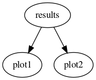
The important point to note is that parameter names determine the dependencies by default.
To address the inflexibility that results from the way we choose to automatically assign dependency, each action is assigned a unique Namespace specification. This allows to specify actions with several different parameters. Let’s make the example above more complicated:
def results(pdf):
    #Compute the results
    ...

def plot1(results, parameter):
    #Take the result and produce a plot of type 1.
    ...

def plot2(results, parameter):
    #Take the result and produce a plot of type 2.
    ...
We can request a parameter scan like this:
pdf: NNPDF30_nlo_as_0118

scan_params:
  - parameter: 5
  - parameter: 10
  - parameter: 20


actions_:
  - scan_params plot1
  - scan_params plot2
which would result in the following computation:

We have requested the two plots to be computed once in each of the three namespaces spanned by scan_params. The actions are in general not computed in the requested namespace, but rather in the outermost one that satisfies all the dependencies (there is also a unique private stack frame per action not shown in the figures above). That’s why, in the graph above, results appears only once: Since it doesn’t depend on the value of parameter (it doesn’t appear in its signature), it is computed in the root namespace, rather than once in each of the scan_params namespaces. If we instead had this:
pdfs:
 - NNPDF30_nlo_as_0118
 - CT14nlo

scan_params:
  - parameter: 5
  - parameter: 10


actions_:
  - pdfs::scan_params plot1
The corresponding graph would be:
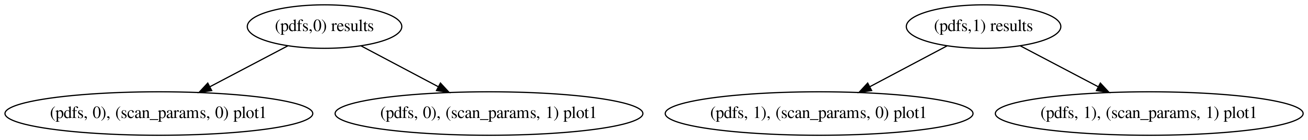
since results does depend on the pdf.
Defining custom pipelines
Here we discuss what needs to go from user entered strings in the YAML file plots and reports.
The basic code flow is as follows:
The
actions_key is parsed to obtain a list of requirements with their associated fuzzyspec.- Each requirement spans other requirements. These can be:
- Providers: Other functions with requirements on their own.
- User input processed by the Configuration, which is immediately tested for correctness.
- Production rules, also derived from the configuration.
Once the requirements are satisfied for a given provider, the checks of the provider are executed.
If all the checks pass, all the runtime requirements are executed in such an order that the dependencies are resolved.
Configuration
A configuration class derived from reportengine.ConfigParser is used to parse the user input. In validphys, it is defined in validphys.Config.
The parsing in reportengine is context dependent. Because we want to specify resources as much as possible before computing anything (at “compile time”), we need to have some information about other resources (e.g. theory folders) in order to do any meaningful processing.
The Config class takes the user input and the dependencies and:
Returns a valid resource if the user input is valid.
Raises a
ConfigErrorif the user input is invalid.
To parse a given user entered key (e.g. posdataset), simply define a parse_posdataset function. The first argument (i.e. second after self) will be the raw value in the configuration file. Any other arguments correspond to dependencies that are already resolved at the point where they are passed to the function (reportengine takes care of that).
For example, we might have:
The type specification (:dict above) makes sure that the user input is of that type before it is seen by the function (which avoids a bunch of repetitive error checking). A positivity dataset requires a theory ID in order to be meaningfully processed (i.e. to find the folder where the fktables are) and therefore the theoryid will be looked for and processed first.
We need to document what the resource we are providing does. The docstring will be seen in validphys --help config:
def parse_posdataset(self, posset:dict, * ,theoryid):
    """An observable used as positivity constrain in the fit.
    It is a mapping containing 'dataset' and 'poslambda'."""
    ...
Production rules
Apart from parse_ functions, which take an explicit user input from the corresponding key (and optionally a set of dependencies), there are the produce_ functions, which take only the dependencies. Other than not taking the user input, the produce_ functions work in a very similar way to the parse_ functions: They are resolved at “compile time”, before any procider function is executed, and they should raise a ConfigError if they fail.
In general production rules should be preferred to parse functions that bundle together various dependencies (e.g. data, cuts and theory), because by having more granular elements, we can iterate over them in different ways: For examples we might want to generate a separate report page for each of the positivity datasets, where they are compared for multiple theories. We could break the parse function above into:
def parse_posdataset_input(self, posset:dict):
    ...

def produce_posdataset(posdataset_input, *, theoryid):
   ...
Now the user has to enter a key called “posdataset_input”, from which some Python object will be obtained as the return value of parse_posdataset_inout. Then, produce_posdataset is used to an object representing the positivity set and the corresponding FKTables in a given theory is obtained from the output of parse_posdataser_input and a theory ID.
Automatically parsing lists
It is possible to easily process list of elements once the parsing for a single element has been defined. Simply add an eleement_of decorator to the parsing function defined in the Config class:
Now posdatasets is parsed as a list of positivity datasets, which can be passed together to a provider, or iterated over, (for example with a with tag in the report, see Report template specification).
Note that you can also put together results from evaluating providers using the collect function, which can be used to map computations over the lists described here.
Validphys loaders
In validphys, we use a Loader class to load resources from various folders. It is good to have a common interface, since it is used to list the available resources of a given type or even download a missing resource. The functions of type check_<resource> should take the information processed by the Config class anf verify that a given resources is correct. If so they should return a “Resouce specification” (something typically containing metadata information such as paths, and a load() method to get the C++ object from libnnpdf). We also define a get method that returns the C++ object directly (although I am not sure it’s very useful anymore).
In the case of the positivity set, this is entirely given in terms of existing check functions:
def check_posset(self, theiryID, setname, postlambda):
    cd = self.check_commondata(setname, 0)
    fk = self.check_fktable(theiryID, setname, [])
    th =  self.check_theoryID(theiryID)
    return PositivitySetSpec(cd, fk, postlambda, th)

def get_posset(self, theiryID, setname, postlambda):
    return self.check_posset(theiryID, setname, postlambda).load()
A more complicated example should raise the appropriate loader errors (see the other examples in the class).
The PositivytySetSpec could be defined roughly like:
 class PositivitySetSpec():
     def __init__(self, commondataspec, fkspec, poslambda, thspec):
         self.commondataspec = commondataspec
         self.fkspec = fkspec
         self.poslambda = poslambda
         self.thspec = thspec

     @property
     def name(self):
         return self.commondataspec.name

     def __str__(self):
         return self.name

     @functools.lru_cache()
     def load(self):
         cd = self.commondataspec.load()
         fk = self.fkspec.load()
         return PositivitySet(cd, fk, self.poslambda)
Here PositivitySet is the libnnpdf object. It is generally better to pass around the spec objects because they are lighter and have more information (e.g. the theory in the above example).
With this, our parser method could look like this:
def parse_posdataset(self, posset:dict, * ,theoryid):
    """An observable used as positivity constrain in the fit.
    It is a mapping containing 'dataset' and 'poslambda'."""
    bad_msg = ("posset must be a mapping with a name ('dataset') and "
               "a float multiplier(poslambda)")

    theoryno, theopath = theoryid
    try:
        name = posset['dataset']
        poslambda = float(posset['poslambda'])
    except KeyError as e:
        raise ConfigError(bad_msg, e.args[0], posset.keys()) from e
    except ValueError as e:
        raise ConfigError(bad_msg) from e

    try:
        return self.loader.check_posset(theoryno, name, poslambda)
    except FileNotFoundError as e:
        raise ConfigError(e) from e
The first part makes sure that the user input is of the expected form (a mapping with a string and a number). The ConfigError has support for suggesting that something could be mistyped. The syntax is ConfigError(message, bad_key, available_keys). For example, if the user enters “poslanda” instead of “postlambda”, the error message would suggest the correct key.
Note that all possible error paths must end by raising a ConfigError.
Computing PDF dependent quantities
Now that we can receive positivity sets as input, let’s do something with them. The SWIG wrappers allow us to call the C++ methods of libnnpdf from Python. These things go in the validphys.results module. We can start by defining a class to produce and hold the results:
class PositivityResult(StatsResult):
    @classmethod
    def from_convolution(cls, pdf, posset):
        loaded_pdf = pdf.load()
        loaded_pos = posset.load()
        data = loaded_pos.GetPredictions(loaded_pdf)
        stats = pdf.stats_class(data.T)
        return cls(stats)

    @property
    def rawdata(self):
        return self.stats.data
pdf.stats_class allows to interpret the results of the convolution as a function of the PDF error type (e.g. to use the different formulas for the uncertainty of Hessian and Monte Carlo sets). In that way it allows to abstract away the different error types. One constructs an object inheriting from validphys.core.Stats that is appropriate for a given error type by calling pdf.stats_class(data) where data is an array where the entries along the first dimension are the results from each member computed from libnnpdf (and the other dimensions are arbitrary). Stats has methods that appropriately collapse along the first axis. For example central_value computes the mean along the first axis for Monte Carlo PDFs and yields the first member for Hesssian PDFs.
And then define a simple provider function:
def positivity_predictions(pdf, positivityset):
     return PositivityResult.from_convolution(pdf, positivityset)
The collect function
In the user interface we have the possibility to perform a computation looping over a list of namespaces. In the code, we can define providers that collect the results of such computations with the collect function.
The signature is:
This will expand the fuzzyspec relative to the current namespace and compute the function once for each frame. Then it will put all the results in a list (to be iterated in the same order as the fuzzyspec) and set that list as the result of the provider. The provider in the first argument is found following the standard reportengine rules. It can be a function defined in a provider module, a configuration input or a production rule, as well as another collect provider. As a special case, one can pass directly functions (defined with the def keyword). For example
Compared to a simple for loop, the collect function has the advantages that the computations are appropriately reused and several results could be computed simultaneously in the parallel mode.
We can use the output of collect as input to other providers. For example:
def count_negative_points(possets_predictions):
    return np.sum([(r.rawdata < 0).sum(axis=1) for r in
        possets_predictions], axis=0)
collect can be used to appropriately group nested inputs. For example here is how to obtain a list of the experiments for each fit.
Note that collect always returns a flat list with the provider evaluated for each of the namespaces spanned by the fuzzyspec. For example
fits_experiments_chi2_flat = collect(abs_chi2_data_experiment,
    ('fits', 'fitcontext', 'experiments',))
results in a flat list containing the result of abs_chi2_data_experiment resolved for each experiment in each fit. One can instead retain the structure by chaining several collect providers. For instance, the code
experiments_chi2 = collect(abs_chi2_data_experiment, ('experiments',))
fits_experiment_chi2_data = collect('experiments_chi2', ('fits', 'fitcontext'))
will result in fits_experiment_chi2_data producing one result for each fit, where each of them is itself list where each item result of abs_chi2_data_experiment evaluated for each experiment in a given fit.
Standard iteration techniques can be used to process the results of collect. For example here is how we would print the χ² for each experiment in each fit:
def print_fits_experiments_chi2(
        fits, fits_experiments, fits_experiment_chi2_data):
    for fit, fit_experiments, experiments_data in zip(
            fits, fits_experiments, fits_experiment_chi2_data):
         print(f"Printing results for {fit}")
         for experiment, chi2data in zip(fit_experiments, experiments_data):
             print(f"χ² for {experiment} is ",
                f"{chi2data.central_result}/{chi2data.ndata}")
A minimal runcard to use the action above is:
fits:
  - NNPDF31_nlo_as_0118
  - NNPDF31_nnlo_as_0118

use_cuts: "fromfit"

actions_:
  - print_fits_experiments_chi2
Checking providers
Providers can checks that verify that all the required preconditions are met. Checks are executed at the time at which the call node is just created and all its required dependencies are either in the namespace or scheduled to be produced. Checking functions take the current state of the namespace, as well as an unspecified set of other parameters (because I haven’t decided on the interface yet!). Therefore check functions should accept **kwargs arguments. Checks are decorated with the reportengine.checks.make_argcheck function. If checks don’t pass, they must raise a reportengine.checks.CheckError exception.
For example, given a reweighting function, we may want to check that the current PDF (the value that will be passed to the function) has a Monte Carlo error type, we might define a check like:
@make_check
def check_pdf_is_montecarlo(ns, **kwargs):
    pdf = ns['pdf']
    etype = pdf.ErrorType
    if etype != 'replicas':
        raise CheckError("Error type of PDF %s must be 'replicas' and not %s"
                          % (pdf, etype))
Checks can be used (abused) to modify the namespace before the action function sees it. This can be used for some advanced context dependent argument default setting (for example setting default file names based on the nsspec).
The check is associated to the provider function by simply applying it as a decorator:
A slightly higher level interface to checks is implemented by the make_argcheck decorator. Instead of receiving a namespace and other unspecified arguments, like the functions decorated with make_check, it simply takes the arguments we want to test. The function can return a dictionary that will be used to update the namespace (but that is not required, it can also not return anything).
For example the check_pdf_is_montecarlo above could be more easily implemented like:
@make_argcheck
def check_pdf_is_montecarlo(pdf):
    etype = pdf.ErrorType
    if etype != 'replicas':
        raise CheckError("Error type of PDF %s must be 'replicas' and not %s"
                          % (pdf, etype))
make_argcheck should be preferred, since it is more explicit, and could be extended with more functionality later on. However it is newer and not very used currently in the code.
Checks have no effect outside of reportengine (unless you call them explicitly).
Ideally, the checks should be sufficient to guarantee that the actions will not fail at runtime.
Producing figures
In order to produce figures, just decorate your functions returning matplotlib Figure objects with the reportengine.figure.figure function, e.g.:
This will take care of the following:
Saving the figures with a nice, unique name to the output folder, in the formats specified by the user.
Closing the figures to save memory.
Making sure figures are properly displayed in reports.
There is also the figuregen decorator for providers that are implemented as generators that yield several figures (see e.g. the implementation of plot_fancy). Apart from just the figure, yield a tuple (prefix, figure) where the prefix will be used in the filename.
Producing tables
These work similarly to figures, as described above. Instead use the @table and @tablegen decorators.
Tables will be saved in the CSV formats.
Customizing how things look in the report
By default, the str() method will be applied to objects that appear in the report. If you want a custom behaviour, declare a declare a custom as_markdown property for your objects. It should return a string in Pandoc Markdown describing your object. Raw HTML is also allowed (although that decreases the compatibility, e.g. if we decide to output LaTeX instead of HTML in the future).
Python static checks and code style
We use Pylint to provide static checking ( e.g. finding basic errors that a compiler would catch in compiled languages) such as uses of unknown variable names, as well as to provide basic guidelines on the structure of the code (e.g. avoid functions that are too complicated). Because Pylint is way too pendantic by default, we limit the checks to only those considered useful. The .pylintrc file at the top level configures Pylint to only mind those checks. Most Python IDEs and editors have some kind of support for pylint. It is strongly recommended to configure the editor to show the problematic pieces of code proactively.
New code should use the Black tool to format the code. This tool should not be used to aggressively reformat existing files.
Example pull request
You may find instructive to go though this pull request that implements arc-length computation:
https://github.com/NNPDF/validphys2/pull/64
It demonstrates how to leverage existing functionality to perform new computations and then present those as plots and tables.
Matplotlib Image Comparison Tests
It is possible to create tests which perform an image comparison between a generated plot and a preexisting baseline plot. Clearly this allows one to check consistency in figure generation.
Before beginning you will need to ensure that you have the tests dependencies, which can be checked in nnpdf/conda-recipe/meta.yml.
The next step is to write the test function. It is highly recommended to use the validphys API for this, both to simplify the code and to make it agnostic to the structure of backend providers - provided that they produce the same results. See for example a function which tests the plot_pdfs provider:
@pytest.mark.mpl_image_compare
def test_plotpdfs():
    pdfs = ['NNPDF31_nnlo_as_0118']
    Q = 10
    flavours = ['g']
    #plot_pdfs returns a generator with (figure, name_hint)
    return next(API.plot_pdfs(pdfs=pdfs, Q=Q, flavours=flavours))[0]
we see that the function needs to return a valid matplotlib figure, and should be decorated with @pytest.mark.mpl_image_compare.
Now the baseline figure needs to be generated, this can be achieved by running
pytest -k <name of file containing test function> --mpl-generate-path=baselinewhich will generated a PNG of the figure in the src/validphys/tests/baseline directory. It is recommended to put all baseline plots in this directory so that they are automatically installed, and so will be in the correct location when the CI runs the test suite.
Now that the baseline figure exists you can check that your test works:
pytest -k <name of file containing test function> --mplAlso you can check that the test has been added to the full test suite:
pytest --pyargs --mpl validphysjust note that if you do not put the --mpl flag then the test will just check that the function runs without error, and won’t check that the output matches to baseline.
Server configuration
Overview
The NNPDF server is a virtual machine (VM) maintained by the Centro Calcolo at the physics department of the University of Milan. The machine has 2 CPUs, 4GB of RAM, 1 TB of disk and it is running CentOS7.
The full disk is backed up every week by the Centro Calcolo. We perform every Sunday a rsync from the /home/nnpdf folder to the nnpdf@lxplus account at CERN.
URLs
The URLs served by this VM are:
- https://data.nnpdf.science: contain public NNPDF data such as PDF fits, releases etc.
- https://vp.nnpdf.science: contains the
validphysreports. - https://wiki.nnpdf.science: with the github wiki version.
- https://packages.nnpdf.science/: The
condabinary packages.
The domain is hosted by Namecheap, which also manages the DNS entries. For each subdomain there is an A record always pointing to the same server IP, currently 159.149.47.24. The subdomains are then handled as described in Web server. For example, a DNS query for packages.nnpdf.science returns
 $ dig packages.nnpdf.science

; <<>> DiG 9.11.3-1ubuntu1.7-Ubuntu <<>> packages.nnpdf.science
;; global options: +cmd
;; Got answer:
;; ->>HEADER<<- opcode: QUERY, status: NOERROR, id: 26766
;; flags: qr rd ra; QUERY: 1, ANSWER: 1, AUTHORITY: 0, ADDITIONAL: 1

;; OPT PSEUDOSECTION:
; EDNS: version: 0, flags:; udp: 65494
;; QUESTION SECTION:
;packages.nnpdf.science.        IN  A

;; ANSWER SECTION:
packages.nnpdf.science. 1799    IN  A   159.149.47.24

;; Query time: 170 msec
;; SERVER: 127.0.0.53#53(127.0.0.53)
;; WHEN: Tue May 28 14:26:53 BST 2019
;; MSG SIZE  rcvd: 67
Access
The access to the server is provided by ssh/vp-upload with the following restrictions:
sshaccess torootis forbidden.- there is a shared
nnpdfuser with low privileges. In order to login the user must send his public ssh key (usually in~/.ssh/id_rsa.pub) to SC. Thennpdfis not allowed to login with password.
The nnpdf user shares a common /home/nnpdf folder where all NNPDF material is stored. Public access to data is available for all files in the /home/nnpdf/WEB folder. The validphys reports are stored in /home/nnpdf/WEB/validphys-reports and the wiki in /home/nnpdf/WEB/wiki.
The conda packages are automatically uploaded to the server by the Continous Integration service (Travis), through an user called dummy which has further reduction in privileges (it uses the rssh shell) and it is only allowed to run the scp command. An accepted private key is stored securely in the Travis configuration under the NNPDF_SSH_KEY variable. It is encoded using base64 because Travis does not easily accept multiline variables. To use it, do something like echo "$NNPDF_SSH_KEY" | base64 --decode. The packages are uploaded to /home/nnpdf/packages.
Web server
We are using nginx as a lightweight and simple web server engine. The nginx initial configuration depends on the linux distribution in use. Usually debian packages provide a ready-to-go version where the /etc/nginx/nginx.conf is already set to work with server blocks (subdomains).
Other distributions like CentOS7 requires more gymnastics, here some tricks:
- make sure the
/home/nnpdffolder can be accessed by thenginxuser - folders served by
nginxmust have permission 755 - create 2 folders in
/etc/nginx:sites-availableandsites-enabled. - in the
/etc/nginx/nginx.conffile indicate the new include path withinclude /etc/nginx/sites-enabled/*;and remove all location statements. - for each server block create a new file in
/etc/nginx/sites-availableand build a symbolic link in/etc/nginx/sites-enabled. - remember to perform a
sudo service nginx restartorsudo nginx -s reloadto update the server block configuration.
Finally, here an example of nginx configuration for the vp.nnpdf.science server block without ssl encryption:
server {
    listen  80;
    listen [::]:80;
    server_name vp.nnpdf.science;

    root /home/nnpdf/WEB/validphys-reports;
    location / {
      try_files $uri $uri/ =404;
        auth_basic "Restricted";
        auth_basic_user_file /home/nnpdf/WEB/validphys-reports/.htpasswd;
    }

    location /thumbnails {
        alias /home/nnpdf/WEB/thumbnails;
        try_files $uri $uri/ =404;
        auth_basic "Restricted";
      auth_basic_user_file /home/nnpdf/WEB/validphys-reports/.htpasswd;
    }
}
Some URLs are password protected using the HTTP basic_auth mechanism. This is implemented by setting the corresponding configuration in nginx, as shown above (specifically with the auth_basic and auth_basic_user_file keys). The .htpasswd files mentioned in the configuration are generated with the htpasswd tool.
SSL encryption
SSL encription is provided by Let’s Encrypt. The certificates are created using the certbot program with the nginx module.
In order to create new ssl certificates, first prepare the nginx server block configuration file and then run the interactive command:
sudo certbot --nginx -d <domain>This will ask you several questions, including if you would like to automatically update the nginx server block file. We fully recommend this approach.
The certificate is automatically renewed by a cron job.
Cron jobs
The following cron jobs are registered for the nnpdf user:
- every day at 4 AM run the
index-email.pyscript. - at every reboot run
index-reports.py,index-fits.py,index-packahes-public.shandindex-packages-private.sh, which monitor contiguously the respective folders and create indexes that can be used by various applications. The first two are homegrown scripts (see Web Scripts) and the later two useconda-index.
The following cron jobs are registered for the root user:
- perform backup of
/home/nnpdfin lxplus every Saturday at noon. - perform a certbot renew every Monday.
- reboot every Sunday at 6am (in order to use new kernels).
- perform system update every day.
Web Scripts
Validphys2 interacts with the NNPDF server by Downloading Resources and Uploading the result.
The server scripts live in the validphys2 repository under the serverscripts folder.
The server side infrastructure that makes this possible currently aims to be minimalistic. The only thing that is done is maintaining some index files (currently for theories, fits, reports and LHAPDF sets) which essentially list the files in a given directory. The indexes are regenerated automatically when their correspondent folders are modified. This is achieved by waiting for changes using the Linux inotify API and my asynwatch module.
The report index is used to display a webpage indexing the reports. It retrieves extra information from a meta.yaml file in the top level output directory, and (with lower priority) by parsing an index.html page contained in the report folder. Properties like title, author and tags are retrieved from the HTML header of this file, and are expected to be in the same format that Pandoc would have used to write them when meta.yaml is passed as a input. To produce it, the most convenient way is setting the main flag of a report, as described in Uploading the result.
Additionally information from the mailing list is added to the index page. Specifically we query the list for links to validphys reports and add links to the emails next to the entries of the reports that are mentioned. This is achieved with the index-email.py script. It needs some authentication credentials to access the mailing list. The password is stored in a file called EMAIL_BOT_PASSWORD, which is not tracked by git. The script outputs two files in the root folder, email_mentions.json which should be used by other applications (such as the report indexer) and seen_emails_cache.pkl, which is there to avoid downloading emails that are already indexes. These files need to be deleted when the format of the index is updated. Currently this script needs to be run manually or as a cron job.
The report index uses the DataTables JS library. It provides filtering and sorting capabilities to the indexes tables. The source file is:
serverscripts/WEB/validphys-reports/index.htmlin the validphys2 directory. It should be updated from time to time to highlight the most interesting reports at a given moment. This can be done by for example displaying in a separate table at the beginning the reports marked with some keyword (for example ‘nnpdf31’).
The Makefile inside will synchronize them with the server.
The report indexing script generates thumbnails in the WEB/thumbnails which are then associated to each report. This is done by looking at the image files inside the figures folder of each uploaded report (see the source of the script for more details). It is expected that the server redirects the requests for vp.nnpdf.science/thumbnails to this folder.
Editing this guide
The source of this document can be found in the main NNPDF repository as the file guide.md, under
doc/validphys2There is a Makefile which will build the HTML document (pandoc and graphviz are required), and make rsync will upload it to the server, if the user has sufficient permissions. Of course, changes to the guide should also be commited to the repository, and if necessary, discussed in a pull request.